Introduction - Preprocessing and visualization of EEG data
Bruno Nicenboim
2024-03-12
Source:vignettes/intro.Rmd
intro.RmdThe package eeguana provides a framework for doing simple
pre-processing with specialized functions and manipulating EEG data with
dplyr verbs (e.g., eeg_mutate,
eeg_filter, eeg_summarize) extended to a new
class eeg_lst, and ggplot wrapper functions.
The new class is inspired by tidyverse principles but it’s not really
“tidy” (due to space considerations), it’s a list of (i) a wide table
that contains the signal amplitudes at every sample point of the EEG,
(ii) an events table with information about markers (or triggers),
blinks and other exported information, and (iii) a long table with
experimental information, such as participant (recording),
conditions, etc.
While it’s possible to transform the eeg_lst to a
data.frame, data.table or a
tibble (with as.data.frame(),
as.data.table() and as_tibble()), the
motivation for manipulating the data in the eeg_lst format
has to do with size considerations. In this case, the original file was
113 MB, converting it to a long format entails a lot of repetition and
generates an object of 556 MB. While this will still work here, a long
format quickly becomes prohibitive in real settings with longer
recordings.
Working with eeguana
Dplyr-like verbs always return an eeg_lst object, which
allows us to use magrittr’s pipe, %>% (see
?`dplyr-eeguana`) or the relatively new R pipe
|>. In addition, eeg_/ch_
functions will also return an eeg_lst unless they have a
suffix _tbl that indicates they return a data frame. In
general, we will work with the eeg_lst, unless we want to
modify the channels information (with channels_tbl()) or
the events table containing markers, artifacts ans custom annotations
(with events_tbl).
A practical example: the N170 effect
Here, I exemplify the use of eeguana with raw EEG data exported in the format of BrainVision 1.0. The data belong to a simple experiment where a participant was presented 100 faces and 100 assorted images in random order. The task of the experiment was to mentally count the number of faces.
First we download the data:
# Run the following or just download the files from raw_faces folder in https://osf.io/tbwvz/
library(httr)
GET("https://osf.io/wv5hp//?action=download",
  write_disk("./s1_faces.vhdr", overwrite = TRUE),
  progress()
)
GET("https://osf.io/c8wea//?action=download",
  write_disk("./s1_faces.vmrk", overwrite = TRUE),
  progress()
)
GET("https://osf.io/uhsde//?action=download",
  write_disk("./s1_faces.eeg", overwrite = TRUE),
  progress()
)
BrainVision 1.0 exports three files: s1_faces.vhdr,
s1_faces.vmrk, and s1_faces.eeg. The file
s1_faces.vhdr contains the metadata and links to the other
two files, s1_faces.vmrk contains the triggers and other
events in the samples, and s1_faces.eeg contains the
signals at every sample for every channel recorded.
We load the relevant packages first. Here, I use
tidytable which is a faster alternative to
dplyr with a very similar interface.
library(tidytable) #or library(dplyr)
library(ggplot2)
library(stringr)
library(eeguana)
set.seed(123) # ICA will always find the same components
We first need to read the data:
faces <- read_vhdr("s1_faces.vhdr")
#> # Reading file s1_faces.vhdr...
#> # Data from ./s1_faces.eeg was read.
#> # Data from 1 segment(s) and 34 channels was loaded.
#> # Object size in memory 113.4 Mb
The function read_vhdr() creates a list with data frames
for the signal, events, segments information, and incorporates in its
attributes generic EEG information.
faces
#> # EEG data:
#>
#> # Signal table:
#> Key: <.id, .sample>
#>           .id      .sample           Fp1           Fpz           Fp2
#>         <int> <sample_int> <channel_dbl> <channel_dbl> <channel_dbl>
#>      1:     1            1     -17878.56     -8921.395     -14028.81
#>      2:     1            2     -17903.75     -8948.022     -14056.53
#>      3:     1            3     -17916.55     -8961.906     -14070.91
#>      4:     1            4     -17918.17     -8963.691     -14068.63
#>      5:     1            5     -17917.71     -8965.658     -14069.16
#>     ---
#> 424484:     1       424484     -16094.71     -8234.730     -13505.21
#> 424485:     1       424485     -16140.11     -8280.301     -13547.56
#> 424486:     1       424486     -16145.24     -8275.078     -13528.22
#> 424487:     1       424487     -16165.22     -8294.479     -13546.50
#> 424488:     1       424488     -16167.39     -8305.199     -13561.12
#>                    F7            F3            Fz            F4            F8
#>         <channel_dbl> <channel_dbl> <channel_dbl> <channel_dbl> <channel_dbl>
#>      1:     -284.2541    -1378.1467     -8077.128      1167.489    -1663.4490
#>      2:     -303.9134    -1400.6560     -8101.660      1145.292    -1685.9034
#>      3:     -307.1683    -1407.8466     -8114.331      1138.028    -1691.4203
#>      4:     -299.8859    -1401.9985     -8116.114      1139.702    -1683.0713
#>      5:     -294.7915    -1401.2996     -8119.442      1136.373    -1684.2664
#>     ---
#> 424484:      609.9043     -236.9552     -7991.669      1977.146     -162.8618
#> 424485:      603.1918     -311.0485     -8045.019      1938.122     -183.0542
#> 424486:      541.3096     -291.0218     -8032.237      1965.358     -132.3712
#> 424487:      467.7130     -302.0740     -8052.393      1930.877     -180.4978
#> 424488:      576.3062     -319.2688     -8065.579      1927.474     -188.0929
#>                   FC5           FC1           FC2           FC6            M1
#>         <channel_dbl> <channel_dbl> <channel_dbl> <channel_dbl> <channel_dbl>
#>      1:     -2315.080     -9040.689     -795.0549     -3665.146             0
#>      2:     -2338.859     -9064.137     -816.1298     -3688.133             0
#>      3:     -2343.475     -9071.438     -823.4675     -3690.046             0
#>      4:     -2333.746     -9065.608     -817.9690     -3681.642             0
#>      5:     -2326.648     -9061.397     -817.2882     -3679.563             0
#>     ---
#> 424484:     -2290.511     -9349.164     -318.8641     -2805.395             0
#> 424485:     -2424.133     -9410.679     -364.1038     -2833.090             0
#> 424486:     -2291.431     -9379.728     -342.3297     -2811.445             0
#> 424487:     -2361.589     -9381.456     -358.2924     -2868.325             0
#> 424488:     -2368.595     -9409.171     -363.8277     -2853.797             0
#>                    T7            C3            Cz            C4            T8
#>         <channel_dbl> <channel_dbl> <channel_dbl> <channel_dbl> <channel_dbl>
#>      1:     -5156.998     -2466.320    -1568.4097     -4427.577    -10351.511
#>      2:     -5184.417     -2490.411    -1591.3053     -4450.049    -10372.402
#>      3:     -5186.146     -2495.726    -1597.7970     -4454.775    -10378.323
#>      4:     -5174.358     -2487.358    -1591.5627     -4449.590    -10373.983
#>      5:     -5170.146     -2481.878    -1588.5833     -4446.334    -10370.489
#>     ---
#> 424484:     -3703.158     -2301.288     -395.4219     -2952.459     -9502.499
#> 424485:     -3834.959     -2372.439     -444.3945     -2994.426     -9465.224
#> 424486:     -3773.260     -2312.064     -419.6414     -2975.410     -9389.198
#> 424487:     -3746.392     -2304.304     -426.3353     -2986.242     -9369.264
#> 424488:     -3615.768     -2358.720     -437.9209     -2984.145     -9521.864
#>                    M2           CP5           CP1           CP2           CP6
#>         <channel_dbl> <channel_dbl> <channel_dbl> <channel_dbl> <channel_dbl>
#>      1:     -1845.363     -8938.128     -4755.838    -1369.6688     -1729.708
#>      2:     -1850.862     -8963.231     -4778.917    -1391.3324     -1750.029
#>      3:     -1845.087     -8969.171     -4784.986    -1397.7506     -1757.532
#>      4:     -1836.370     -8957.989     -4775.938    -1391.9026     -1754.553
#>      5:     -1841.961     -8950.726     -4772.205    -1388.7207     -1755.197
#>     ---
#> 424484:     -2128.771     -8037.571     -4200.332     -677.7635     -1046.501
#> 424485:     -2179.546     -8083.840     -4253.405     -721.7708     -1080.431
#> 424486:     -2153.340     -8027.603     -4225.636     -702.5348     -1048.874
#> 424487:     -2141.644     -8046.398     -4230.160     -709.1735     -1040.856
#> 424488:     -2130.978     -8060.742     -4244.541     -712.0606     -1053.931
#>                    P7            P3            Pz            P4            P8
#>         <channel_dbl> <channel_dbl> <channel_dbl> <channel_dbl> <channel_dbl>
#>      1:     -7513.455     -8512.474    -537.63159     -99.10343     -875.6397
#>      2:     -7535.836     -8533.438    -557.97095    -117.14455     -892.3933
#>      3:     -7541.739     -8537.741    -561.55725    -122.82701     -892.9816
#>      4:     -7530.282     -8529.099    -552.78510    -117.75130     -886.6740
#>      5:     -7524.361     -8523.562    -549.19885    -117.82441     -885.3681
#>     ---
#> 424484:     -5433.473     -8150.485     -34.94090     496.89807     -182.1897
#> 424485:     -5470.565     -8197.932     -79.35287     458.84891     -229.4153
#> 424486:     -5474.501     -8173.215     -60.83399     476.24600     -226.5095
#> 424487:     -5488.533     -8182.244     -64.40166     471.66693     -247.6580
#> 424488:     -5478.491     -8187.780     -69.53255     475.47369     -247.5108
#>                   POz            O1            Oz            O2          HEOG
#>         <channel_dbl> <channel_dbl> <channel_dbl> <channel_dbl> <channel_dbl>
#>      1:     -852.6708     -4117.080     -1950.149     -817.4540     -5006.420
#>      2:     -871.1710     -4136.997     -1965.578     -825.3984     -5027.017
#>      3:     -873.9114     -4138.725     -1965.137     -824.5893     -5037.775
#>      4:     -866.0771     -4126.606     -1957.450     -823.7434     -5033.031
#>      5:     -865.5070     -4127.543     -1967.270     -834.0415     -5031.210
#>     ---
#> 424484:     -304.2810     -2730.290     -1170.744      -67.8408     -3137.224
#> 424485:     -345.6953     -2777.571     -1209.235     -104.1242     -3216.466
#> 424486:     -342.8815     -2794.121     -1232.792     -135.4974     -3136.874
#> 424487:     -343.4331     -2790.444     -1224.516     -152.9679     -3105.096
#> 424488:     -350.5685     -2804.640     -1245.077     -186.8792     -3162.988
#>                  VEOG
#>         <channel_dbl>
#>      1:     -9116.806
#>      2:     -9133.780
#>      3:     -9138.781
#>      4:     -9134.222
#>      5:     -9139.996
#>     ---
#> 424484:     -8591.514
#> 424485:     -8672.283
#> 424486:     -8648.578
#> 424487:     -8658.159
#> 424488:     -8660.311
#>
#> # Events table:
#>        .id       .type .description     .initial       .final .channel
#>      <int>      <char>       <char> <sample_int> <sample_int>   <char>
#>   1:     1 New Segment                         1            1     <NA>
#>   2:     1    Stimulus         s111        10528        10528     <NA>
#>   3:     1    Stimulus         s130        10742        10742     <NA>
#>   4:     1    Stimulus          s71        11175        11175     <NA>
#>   5:     1    Stimulus         s130        12806        12806     <NA>
#>  ---
#> 401:     1    Stimulus         s130       411197       411197     <NA>
#> 402:     1    Stimulus          s71       411469       411469     <NA>
#> 403:     1    Stimulus         s121       412943       412943     <NA>
#> 404:     1    Stimulus         s122       412966       412966     <NA>
#> 405:     1    Stimulus         s102       412989       412989     <NA>
#>
#> # Segments table:
#> Key: <.id>
#>      .id    .recording segment
#>    <int>        <char>   <int>
#> 1:     1 s1_faces.vhdr       1
summary(faces)
#> # EEG data:
#> # Sampling rate: 512 Hz.
#> # Size in memory: 113.4 Mb.
#> # Total duration: 00:13:49.
#> # Summary of segments
#>       .recording n_segments n_incomplete
#>           <char>      <int>        <int>
#> 1: s1_faces.vhdr          1            0
#> # Summary of events
#>          .type .description     n
#>         <char>       <char> <int>
#> 1: New Segment                  1
#> 2:    Stimulus         s102     1
#> 3:    Stimulus         s111     1
#> 4:    Stimulus         s121     1
#> 5:    Stimulus         s122     1
#> 6:    Stimulus         s130   200
#> 7:    Stimulus          s70   100
#> 8:    Stimulus          s71   100
We see that there is no electrode positions in the object, but since
we know that the layout was a standard 10/20, we’ll add this layout to
the object, using the dataset layout_32_1020. This is
required to be able to create topographic plots.
channels_tbl(faces)
#> .channel number .reference resolution unit radius theta phi .x
#> <char> <char> <char> <num> <char> <num> <num> <num> <num>
#> 1: Fp1 Ch1 <NA> 1 microvolts NA NA NA NA
#> 2: Fpz Ch2 <NA> 1 microvolts NA NA NA NA
#> 3: Fp2 Ch3 <NA> 1 microvolts NA NA NA NA
#> 4: F7 Ch4 <NA> 1 microvolts NA NA NA NA
#> 5: F3 Ch5 <NA> 1 microvolts NA NA NA NA
#> 6: Fz Ch6 <NA> 1 microvolts NA NA NA NA
#> 7: F4 Ch7 <NA> 1 microvolts NA NA NA NA
#> 8: F8 Ch8 <NA> 1 microvolts NA NA NA NA
#> 9: FC5 Ch9 <NA> 1 microvolts NA NA NA NA
#> 10: FC1 Ch10 <NA> 1 microvolts NA NA NA NA
#> 11: FC2 Ch11 <NA> 1 microvolts NA NA NA NA
#> 12: FC6 Ch12 <NA> 1 microvolts NA NA NA NA
#> 13: M1 Ch13 <NA> 1 microvolts NA NA NA NA
#> 14: T7 Ch14 <NA> 1 microvolts NA NA NA NA
#> 15: C3 Ch15 <NA> 1 microvolts NA NA NA NA
#> 16: Cz Ch16 <NA> 1 microvolts NA NA NA NA
#> 17: C4 Ch17 <NA> 1 microvolts NA NA NA NA
#> 18: T8 Ch18 <NA> 1 microvolts NA NA NA NA
#> 19: M2 Ch19 <NA> 1 microvolts NA NA NA NA
#> 20: CP5 Ch20 <NA> 1 microvolts NA NA NA NA
#> 21: CP1 Ch21 <NA> 1 microvolts NA NA NA NA
#> 22: CP2 Ch22 <NA> 1 microvolts NA NA NA NA
#> 23: CP6 Ch23 <NA> 1 microvolts NA NA NA NA
#> 24: P7 Ch24 <NA> 1 microvolts NA NA NA NA
#> 25: P3 Ch25 <NA> 1 microvolts NA NA NA NA
#> 26: Pz Ch26 <NA> 1 microvolts NA NA NA NA
#> 27: P4 Ch27 <NA> 1 microvolts NA NA NA NA
#> 28: P8 Ch28 <NA> 1 microvolts NA NA NA NA
#> 29: POz Ch29 <NA> 1 microvolts NA NA NA NA
#> 30: O1 Ch30 <NA> 1 microvolts NA NA NA NA
#> 31: Oz Ch31 <NA> 1 microvolts NA NA NA NA
#> 32: O2 Ch32 <NA> 1 microvolts NA NA NA NA
#> 33: HEOG Ch33 <NA> 1 microvolts NA NA NA NA
#> 34: VEOG Ch34 <NA> 1 microvolts NA NA NA NA
#> .channel number .reference resolution unit radius theta phi .x
#> .y .z
#> <num> <num>
#> 1: NA NA
#> 2: NA NA
#> 3: NA NA
#> 4: NA NA
#> 5: NA NA
#> 6: NA NA
#> 7: NA NA
#> 8: NA NA
#> 9: NA NA
#> 10: NA NA
#> 11: NA NA
#> 12: NA NA
#> 13: NA NA
#> 14: NA NA
#> 15: NA NA
#> 16: NA NA
#> 17: NA NA
#> 18: NA NA
#> 19: NA NA
#> 20: NA NA
#> 21: NA NA
#> 22: NA NA
#> 23: NA NA
#> 24: NA NA
#> 25: NA NA
#> 26: NA NA
#> 27: NA NA
#> 28: NA NA
#> 29: NA NA
#> 30: NA NA
#> 31: NA NA
#> 32: NA NA
#> 33: NA NA
#> 34: NA NA
#> .y .z
## In case the order of the electrodes is different, we do a left_join instead of replacing the table:
channels_tbl(faces) <- select(channels_tbl(faces), .channel) |>
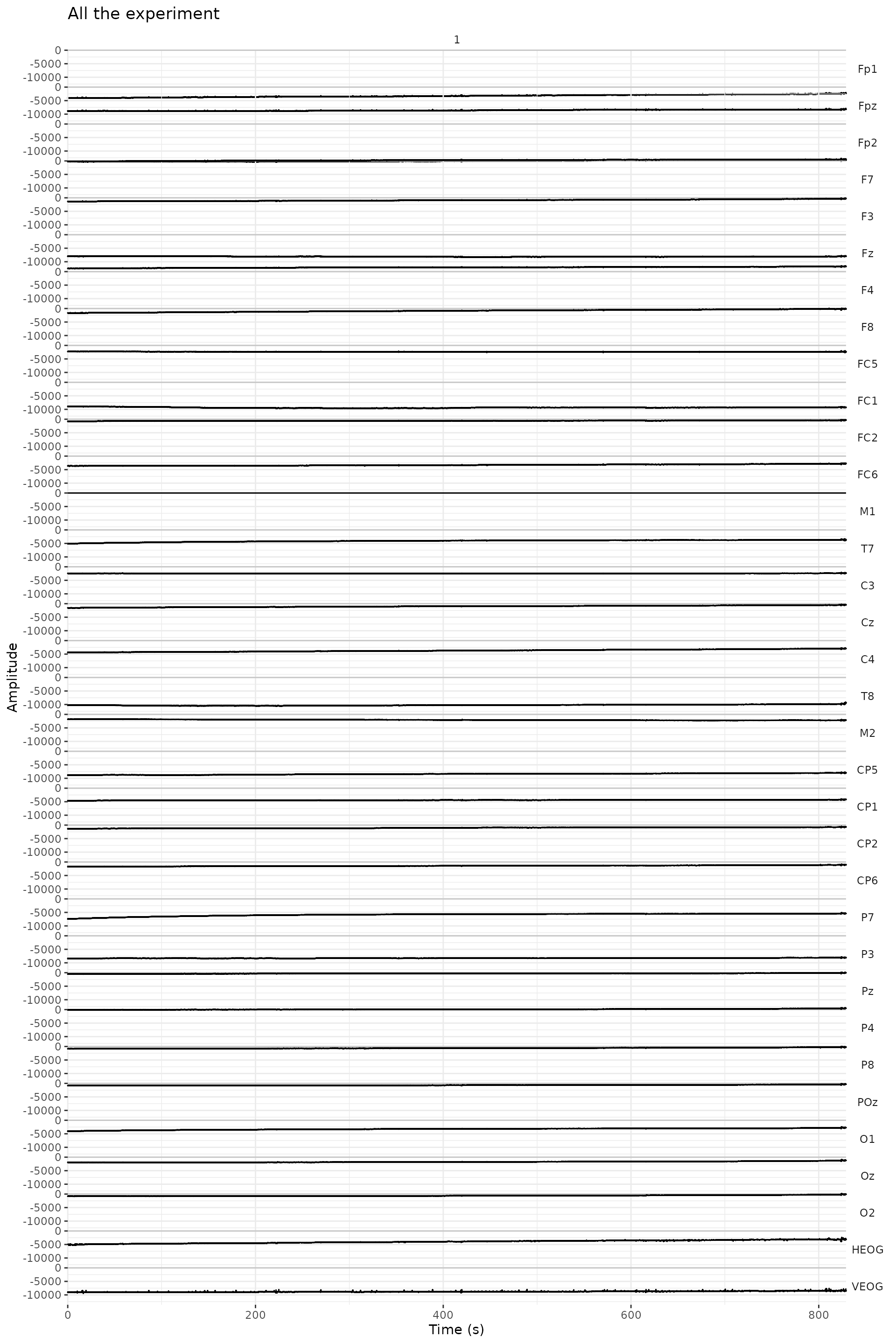
left_join(layout_32_1020)The plots that eeguana produce are
ggplot objects that can be modified like regular
ggplot.
plot(faces) +
  ggtitle("All the experiment")
#> # Downsampling from 512Hz to 256Hz.
#> # Object size in memory 56.7 Mb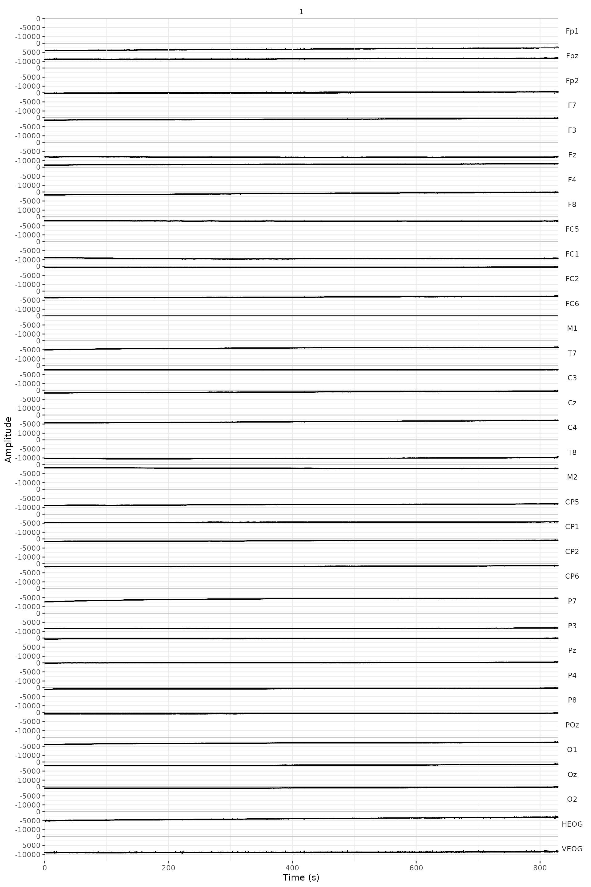
Pre-processing
Here the preprocessing is done with only one EEG dataset. If the EEG
data of different participants is available, one can repeat a similar
preprocessing pipeline for each dataset and bind the EEG datasets with
bind().
Rereferencing
In this dataset, the signal from all electrodes is monopolar and referenced to the left mastoid (M1). We want the signal (excluding the EOG channels) to be referenced to linked (left and right) mastoids (M1 and M2).
faces <- eeg_rereference(faces, -VEOG, -HEOG, .ref = c("M1", "M2"))Filtering
We apply a band pass filter of 0.1 to 30 Hz to all the channels except the EOG channels. We don’t segment yet, because discontinuities in the signal create artifacts on the edges.
faces_filt <- eeg_filt_band_pass(faces, -HEOG, -VEOG, .freq = c(.1, 30))
#> Setting up band-pass filter from 0.1 - 30 Hz
#> Width of the transition band at the low cut-off frequency is 0.1 Hz
#> Width of the transition band at the high cut-off frequency is 7.5 Hz
ICA
We want to apply ICA to as much data as possible, but to “representative” data: to data of the experiment and not when the participants were moving or reading the instructions. For the same reason, we want to the ignore artifacts that we are sure are not representing brain activity, because of the extreme amplitudes in the signal.
We first cut a large segment that excludes data before and after the
experiment was ran using eeg_segment() (that is, only data
from the marker “s111” to “s121”), and then we mark differences of 200
microvolts between peaks with eeg_artif_minmax().
faces_ls <- eeg_segment(faces_filt,
.description == "s111",
.end = .description == "s121") |>
eeg_artif_minmax(-HEOG, -VEOG,
.threshold = 200,
.window = 200,
.unit = "ms")
#> # Total of 1 segments found.
#> # Object size in memory 107.5 Mb after segmentation.
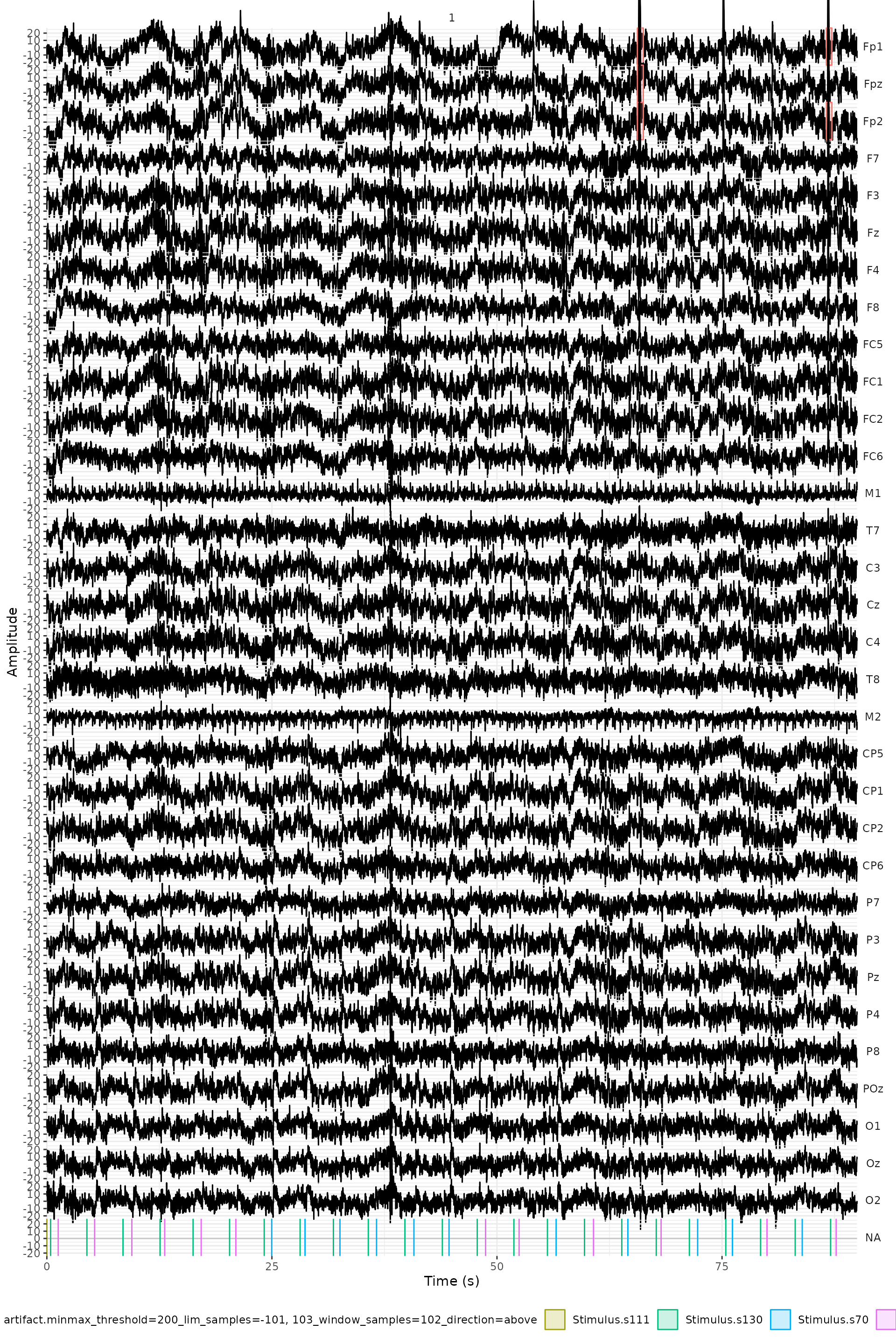
#> # Number of intervals with artifacts: 118eeg_artif_minimax() only adds the artifacts in the
events table and doesn’t modify the signal. We can have a look at the
type of artifacts that were detected, by plotting the signal and the
events with annotate_events(). It would be a good idea to
just check a couple of seconds of the signal, for that we use the
dplyr-like function eeg_filter().
faces_ls |>
  eeg_select(-HEOG, -VEOG)|>
  eeg_filter(as_time(.sample, .unit = "s") |> between(0, 90)) |>
  plot() +
  annotate_events() +
  theme(legend.position = "bottom")
#> # Downsampling from 512Hz to 256Hz.
#> # Object size in memory 5.9 Mb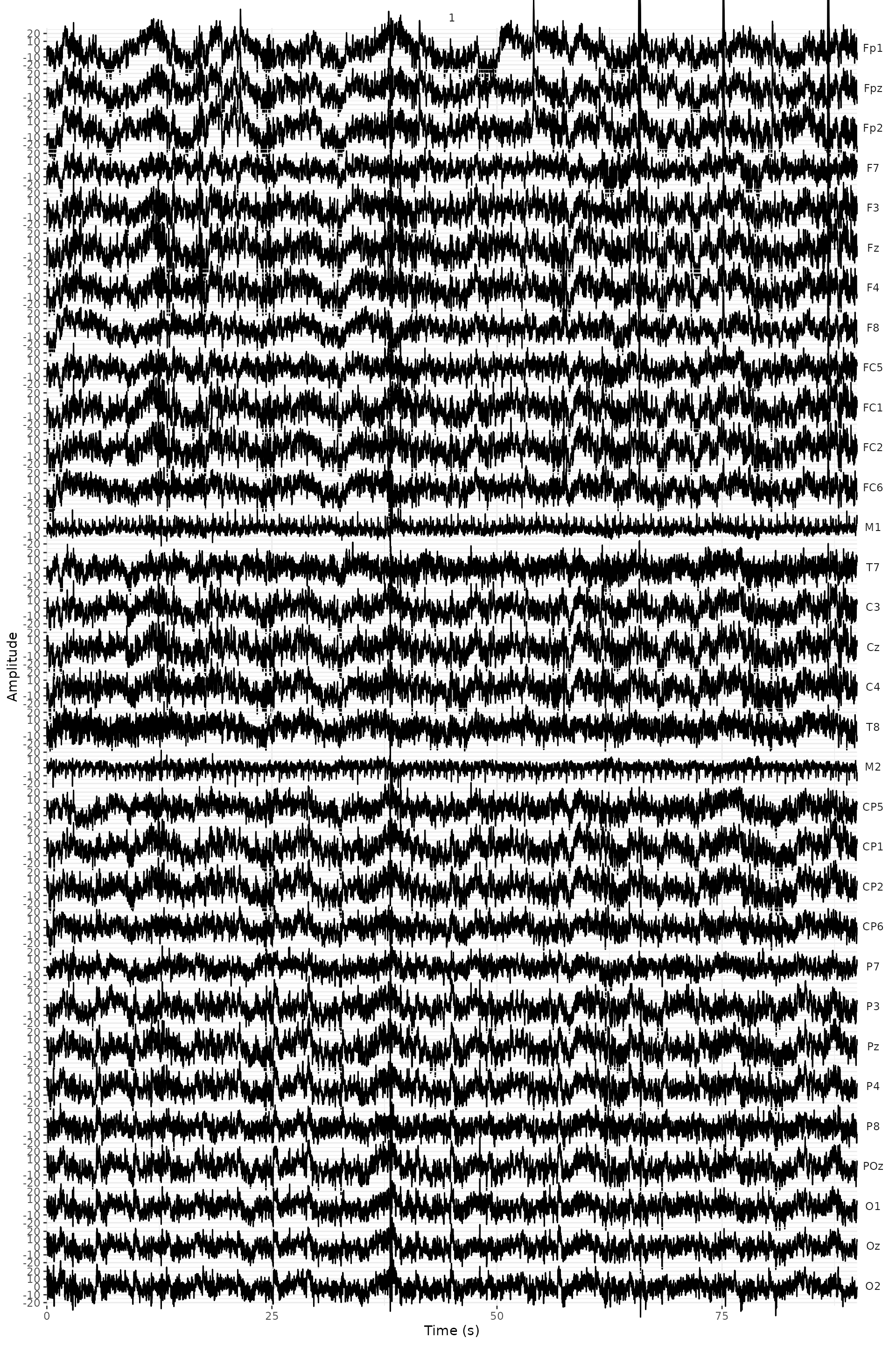
Now we can run ICA, removing the EOG and reference electrodes, and ignoring the artifacts.
## By default, it will ignore artifacts
faces_ica <- faces_ls |>
  eeg_ica(-HEOG, -VEOG, -M1, -M2, .method = adapt_fast_ICA, .ignore = .type == "artifact")
#> # ICA is being done using adapt_fast_ICA...
#> # 97% of the samples will be used.
#> # ICA took 59.58 secs
We can now check the different topographic plots of the ICAs with
plot_components(), and their correlation with the EOG
channels looking a the summary of the object.
faces_ica |> plot_components()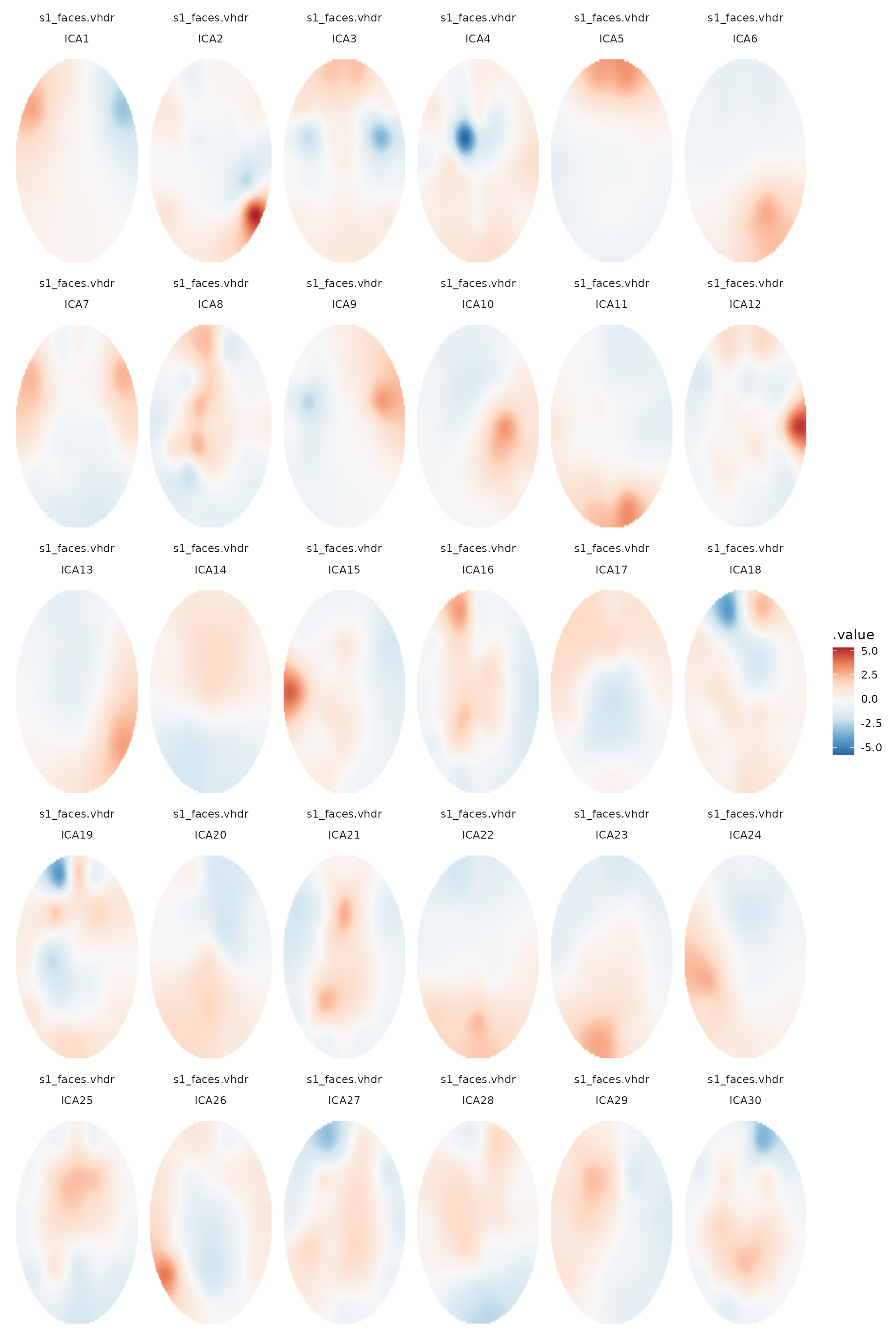
eeg_ica_summary_tbl(faces_ica)
#> EOG channels detected as: HEOG, VEOG
#> # Downsampling from 512Hz to 256Hz.
#> # Object size in memory 53.8 Mb
#>        .recording    EOG   .ICA           cor           var
#>            <char> <char> <char>         <num>         <num>
#>  1: s1_faces.vhdr   VEOG   ICA5  0.3110616894  3.757060e-01
#>  2: s1_faces.vhdr   HEOG   ICA5  0.0060600201  3.757060e-01
#>  3: s1_faces.vhdr   VEOG  ICA14  0.0594109202  7.014123e-02
#>  4: s1_faces.vhdr   HEOG  ICA14  0.0115211860  7.014123e-02
#>  5: s1_faces.vhdr   VEOG  ICA25  0.0191137136  5.700112e-02
#>  6: s1_faces.vhdr   HEOG  ICA25  0.0079409656  5.700112e-02
#>  7: s1_faces.vhdr   VEOG  ICA28  0.0215901453  5.238918e-02
#>  8: s1_faces.vhdr   HEOG  ICA28 -0.0026613292  5.238918e-02
#>  9: s1_faces.vhdr   VEOG  ICA13 -0.0733915975  4.883691e-02
#> 10: s1_faces.vhdr   HEOG  ICA13  0.0028042746  4.883691e-02
#> 11: s1_faces.vhdr   VEOG  ICA16  0.0189808192  3.920680e-02
#> 12: s1_faces.vhdr   HEOG  ICA16 -0.0052139432  3.920680e-02
#> 13: s1_faces.vhdr   VEOG  ICA27 -0.0146958686  3.894493e-02
#> 14: s1_faces.vhdr   HEOG  ICA27 -0.0005737728  3.894493e-02
#> 15: s1_faces.vhdr   HEOG  ICA26 -0.0127623329  3.356974e-02
#> 16: s1_faces.vhdr   VEOG  ICA26 -0.0103929696  3.356974e-02
#> 17: s1_faces.vhdr   VEOG  ICA21 -0.0110379588  3.209207e-02
#> 18: s1_faces.vhdr   HEOG  ICA21  0.0041385932  3.209207e-02
#> 19: s1_faces.vhdr   VEOG  ICA30 -0.0318988532  3.195685e-02
#> 20: s1_faces.vhdr   HEOG  ICA30 -0.0049492927  3.195685e-02
#> 21: s1_faces.vhdr   HEOG  ICA11 -0.0080689883  1.531692e-02
#> 22: s1_faces.vhdr   VEOG  ICA11 -0.0022034332  1.531692e-02
#> 23: s1_faces.vhdr   VEOG   ICA8 -0.0061078333  1.503484e-02
#> 24: s1_faces.vhdr   HEOG   ICA8 -0.0033160702  1.503484e-02
#> 25: s1_faces.vhdr   VEOG  ICA22 -0.0729992398  1.342674e-02
#> 26: s1_faces.vhdr   HEOG  ICA22 -0.0075857794  1.342674e-02
#> 27: s1_faces.vhdr   VEOG  ICA19 -0.0113037545  1.276725e-02
#> 28: s1_faces.vhdr   HEOG  ICA19  0.0040990970  1.276725e-02
#> 29: s1_faces.vhdr   HEOG  ICA29 -0.0098960226  1.268456e-02
#> 30: s1_faces.vhdr   VEOG  ICA29  0.0082034132  1.268456e-02
#> 31: s1_faces.vhdr   VEOG  ICA10  0.0029772146  1.075145e-02
#> 32: s1_faces.vhdr   HEOG  ICA10 -0.0012705350  1.075145e-02
#> 33: s1_faces.vhdr   VEOG  ICA23 -0.0139531104  1.074641e-02
#> 34: s1_faces.vhdr   HEOG  ICA23  0.0080386572  1.074641e-02
#> 35: s1_faces.vhdr   VEOG   ICA1  0.0590125612  9.976911e-03
#> 36: s1_faces.vhdr   HEOG   ICA1 -0.0556782278  9.976911e-03
#> 37: s1_faces.vhdr   VEOG   ICA2 -0.0126428949  7.926289e-03
#> 38: s1_faces.vhdr   HEOG   ICA2 -0.0078820112  7.926289e-03
#> 39: s1_faces.vhdr   VEOG  ICA24 -0.0121801971  4.817679e-03
#> 40: s1_faces.vhdr   HEOG  ICA24 -0.0016042248  4.817679e-03
#> 41: s1_faces.vhdr   HEOG   ICA7 -0.0020891334  3.213752e-03
#> 42: s1_faces.vhdr   VEOG   ICA7 -0.0003910153  3.213752e-03
#> 43: s1_faces.vhdr   VEOG  ICA12  0.0144307012  1.612964e-03
#> 44: s1_faces.vhdr   HEOG  ICA12  0.0128083915  1.612964e-03
#> 45: s1_faces.vhdr   HEOG  ICA17 -0.0091874914  1.242015e-03
#> 46: s1_faces.vhdr   VEOG  ICA17  0.0017426840  1.242015e-03
#> 47: s1_faces.vhdr   VEOG  ICA18 -0.0131764353  8.322457e-04
#> 48: s1_faces.vhdr   HEOG  ICA18 -0.0117696565  8.322457e-04
#> 49: s1_faces.vhdr   HEOG   ICA4 -0.0190202998  5.031454e-04
#> 50: s1_faces.vhdr   VEOG   ICA4 -0.0171506626  5.031454e-04
#> 51: s1_faces.vhdr   VEOG   ICA6 -0.0089105463  4.392834e-05
#> 52: s1_faces.vhdr   HEOG   ICA6  0.0049753303  4.392834e-05
#> 53: s1_faces.vhdr   VEOG  ICA20 -0.0062150226  1.952812e-06
#> 54: s1_faces.vhdr   HEOG  ICA20 -0.0011994425  1.952812e-06
#> 55: s1_faces.vhdr   HEOG   ICA9 -0.0019097967 -4.193406e-04
#> 56: s1_faces.vhdr   VEOG   ICA9  0.0015343447 -4.193406e-04
#> 57: s1_faces.vhdr   VEOG  ICA15 -0.0265727074 -1.012186e-03
#> 58: s1_faces.vhdr   HEOG  ICA15 -0.0041488999 -1.012186e-03
#> 59: s1_faces.vhdr   VEOG   ICA3  0.0866623859 -7.459674e-03
#> 60: s1_faces.vhdr   HEOG   ICA3 -0.0019740756 -7.459674e-03
#>        .recording    EOG   .ICA           cor           var
We’ll look closer at the ICA that are more likely to be related to eye movements, and we’ll compare with signals that look like blinks and saccades:
faces_ica <- faces_ica |>
  eeg_artif_step(HEOG, VEOG,
                 .threshold = 30,
                 .window = 200,
                 .unit = "ms",
                 .freq = c(1, 10)) |>
  eeg_artif_peak(VEOG, .threshold = 100, .freq = c(1, 10))
#> Setting up band-pass filter from 1 - 10 Hz
#> Width of the transition band at the low cut-off frequency is 1 Hz
#> Width of the transition band at the high cut-off frequency is 2.5 Hz
#> # Number of intervals with artifacts: 407
#> Setting up band-pass filter from 1 - 10 Hz
#> Width of the transition band at the low cut-off frequency is 1 Hz
#> Width of the transition band at the high cut-off frequency is 2.5 Hz
#> # Number of intervals with artifacts: 158
In order to investigate the ICA, we are using an experimental
function not yet exported (that’s why we use the :::). This function
will probably converted into a shiny app. It’s possible to get the same
plots by using a combination of plot_topo,
eeg_ica_show, eeg_ica_summary_tbl, and some
ggplot and cowplot functions.
We’ll see how the components explaining the most variance and most correlated to the EOG channels behave:
#samples with blinks
s_peaks <- filter(events_tbl(faces_ica),  str_starts(.description, "peak")) |>
  pull(.initial)
eeguana:::plot_ica.eeg_ica_lst(faces_ica, samples = seq(s_peaks[1]-2000,s_peaks[1]+2000))
#> Warning in eeguana:::plot_ica.eeg_ica_lst(faces_ica, samples = seq(s_peaks[1] -
#> : This is an experimental function, and it might change or disappear in the
#> future. (Or it might be transformed into a shinyapp)
#> Using recording: s1_faces.vhdr
#> EOG channels detected as: HEOG, VEOG
#> Calculating the correlation of ICA components with filtered EOG channels...
#> Setting up band-pass filter from 0.1 - 30 Hz
#> Width of the transition band at the low cut-off frequency is 0.1 Hz
#> Width of the transition band at the high cut-off frequency is 7.5 Hz
#> EOG channels detected as: HEOG, VEOG
#> # Downsampling from 512Hz to 256Hz.
#> # Object size in memory 53.9 Mb
#> The following columns of signal_tbl are not channels (or ICA components): ICA5ICA14ICA25ICA28ICA13ICA16ICA27ICA26ICA21ICA30ICA11ICA8ICA22ICA19ICA29ICA10
#> * To build a channel use `channel_dbl()` function, e.g. channel_dbl(0) to populate the table with a channel containing 0 microvolts.
#> * To copy the structure of an existing channel one can do `new_ch = existing_channel * 0 + ...`
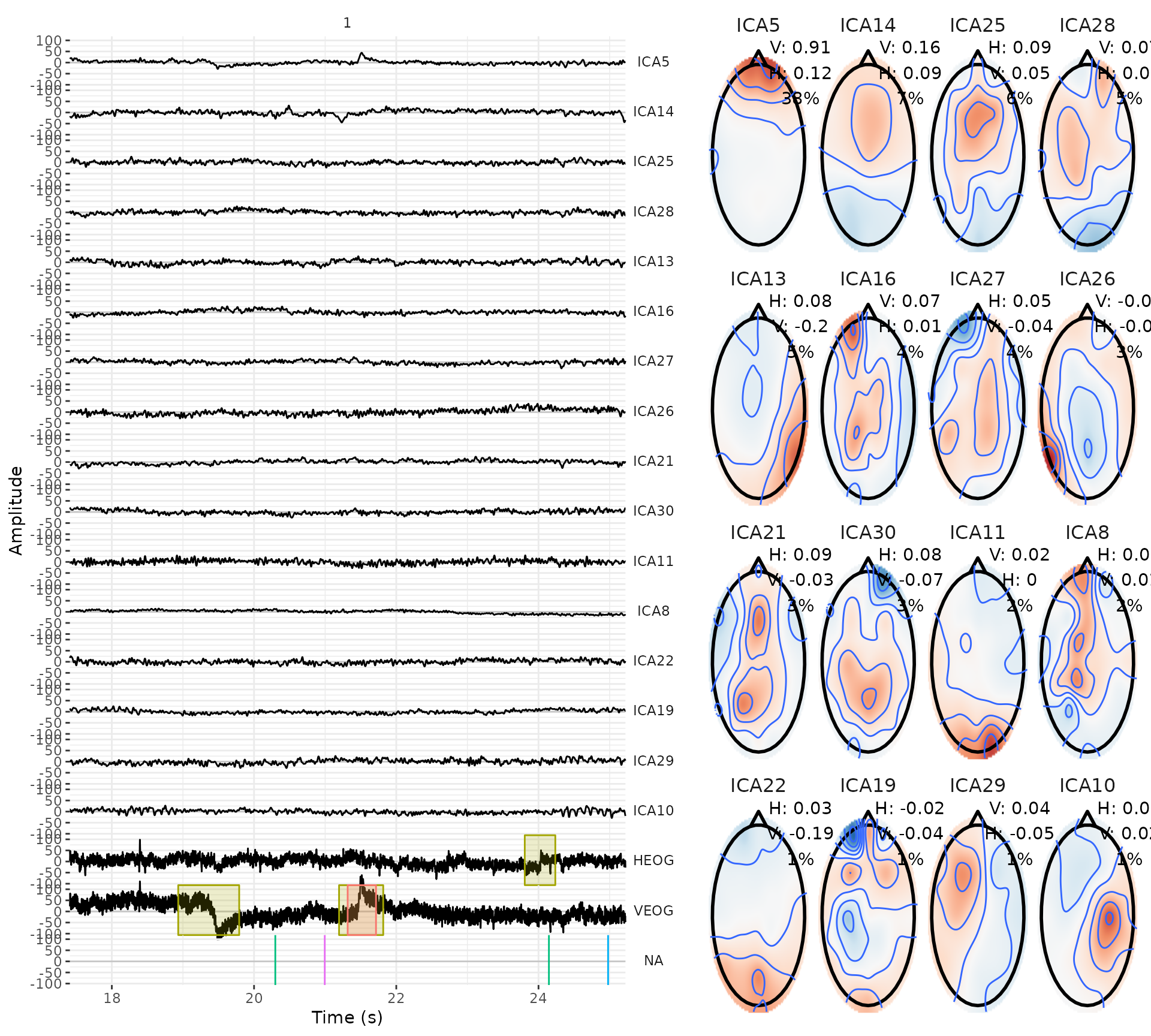
The clearest ones is ICA5, and so we’ll just remove that one.
faces_icaed <- faces_ica |>
  eeg_ica_keep(-ICA5) |>
  as_eeg_lst()
Now we’ll segment the data to appropriate check if there are still artifacts.
events_tbl(faces_icaed) <- events_tbl(faces_icaed) |>
filter(!.type %in% "artifact")
faces_seg <- faces_icaed |>
eeg_select(-description, -type) |>
eeg_segment(.description %in% c("s70", "s71"), .lim = c(-.1, .5))
#> # Total of 200 segments found.
#> # Object size in memory 16.5 Mb after segmentation.
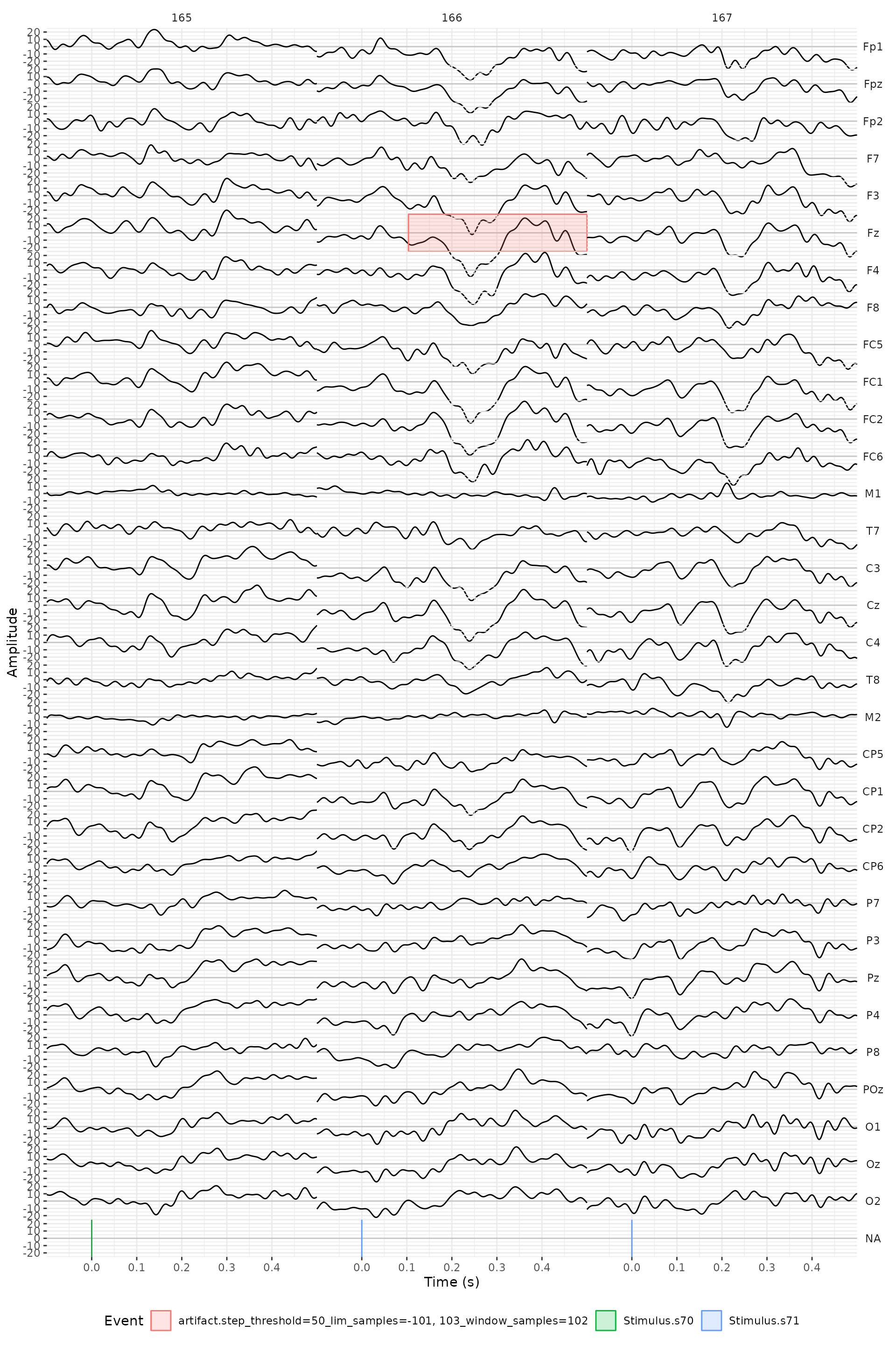
faces_seg_artif <- faces_seg |>
eeg_artif_minmax(-HEOG, -VEOG, .threshold = 100, .window = 150, .unit = "ms") |>
eeg_artif_step(-HEOG, -VEOG, .threshold = 50, .window = 200, .unit = "ms")
#> # Number of intervals with artifacts: 0
#> # Number of intervals with artifacts: 1
## extracts the ids of the segments with artifacts
bad <- filter(events_tbl(faces_seg_artif), .type == "artifact") |>
pull(.id) |>
unique()
## Show the segment with artifact and one before and after:
faces_seg_artif |>
eeg_filter(.id %in% c(bad-1, bad, bad+1)) |>
eeg_select(-VEOG, -HEOG) |>
plot() +
annotate_events() +
theme(legend.position = "bottom")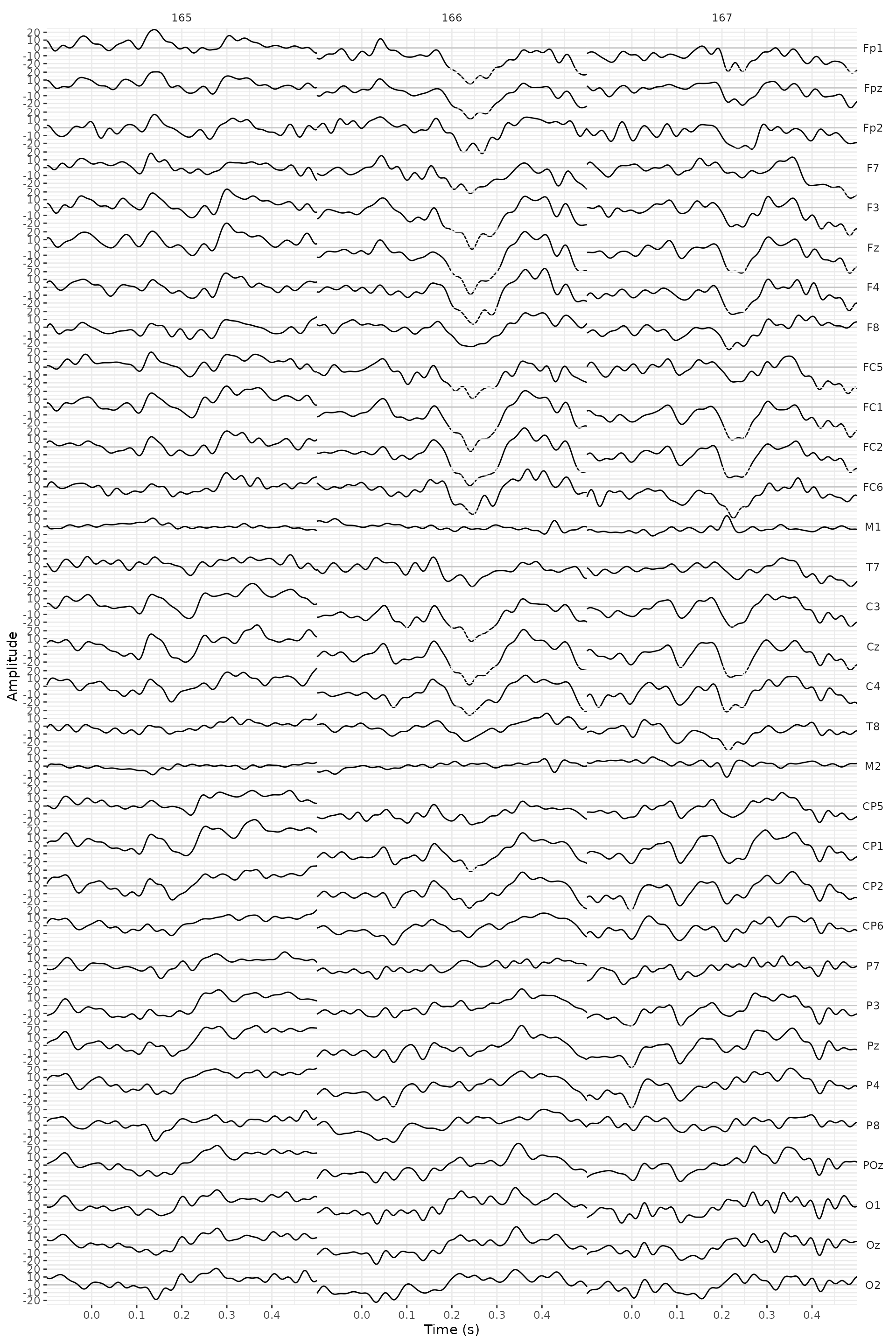
faces_seg <- faces_seg_artif |>
  eeg_events_to_NA(.type == "artifact", .entire_seg = TRUE, .drop_events = TRUE)

summary(faces_seg)
#> # EEG data:
#> # Sampling rate: 512 Hz.
#> # Size in memory: 16.5 Mb.
#> # Total duration: 00:02:00.
#> # Summary of segments
#>       .recording n_segments n_incomplete
#>           <char>      <int>        <int>
#> 1: s1_faces.vhdr        200            1
#> # Summary of events
#>       .type .description     n
#>      <char>       <char> <int>
#> 1: Stimulus          s70   100
#> 2: Stimulus          s71   100
Finally, we can baseline the segments:
faces_seg <- faces_seg |>
  eeg_baseline()
Visualization
We edit the segmentation information and add more descriptive labels.
faces_seg <- faces_seg |>
eeg_mutate(
condition =
ifelse(description == "s70", "faces", "non-faces")
) |>
eeg_select(-type)
faces_seg
#> # EEG data:
#>
#> # Signal table:
#> Key: <.id, .sample>
#> .id .sample Fp1 Fpz Fp2
#> <int> <sample_int> <channel_dbl> <channel_dbl> <channel_dbl>
#> 1: 1 -50 -0.2239737 2.926696 0.1088197
#> 2: 1 -49 0.9975430 3.910457 0.7585352
#> 3: 1 -48 2.2477072 4.853125 1.5129425
#> 4: 1 -47 3.3361201 5.596977 2.2208750
#> 5: 1 -46 4.0950011 6.007830 2.7411833
#> ---
#> 61596: 200 253 -7.4272958 -4.030794 -3.3414518
#> 61597: 200 254 -7.0028675 -4.076854 -3.7139526
#> 61598: 200 255 -6.3948136 -4.124318 -4.0795149
#> 61599: 200 256 -5.7744059 -4.236721 -4.4670174
#> 61600: 200 257 -5.3225204 -4.474952 -4.9176401
#> F7 F3 Fz F4 F8
#> <channel_dbl> <channel_dbl> <channel_dbl> <channel_dbl> <channel_dbl>
#> 1: -0.1107286 3.793132 4.228278 2.840110 -3.15472635
#> 2: 0.7172289 4.038747 4.270218 2.382479 -2.35472265
#> 3: 1.7686192 4.340948 4.421612 2.013301 -1.24644410
#> 4: 2.9135916 4.642705 4.591250 1.709526 0.05225002
#> 5: 4.0297893 4.899710 4.700407 1.452931 1.40978255
#> ---
#> 61596: 2.5704919 4.188729 -8.730353 -12.167556 -1.36556543
#> 61597: 1.3456003 3.356811 -9.453131 -11.842863 -2.17206941
#> 61598: 0.2178476 2.644884 -9.985577 -11.460650 -2.78238153
#> 61599: -0.8343465 1.996052 -10.366157 -11.047480 -3.20156158
#> 61600: -1.8464510 1.323714 -10.661645 -10.644149 -3.46204537
#> FC5 FC1 FC2 FC6 M1
#> <channel_dbl> <channel_dbl> <channel_dbl> <channel_dbl> <channel_dbl>
#> 1: 1.6113910 1.592771 -2.364200 -1.8391090 -2.030141
#> 2: 2.0405680 1.860704 -2.861841 -1.1455898 -1.922150
#> 3: 2.4513040 2.219617 -3.123105 -0.1976263 -1.785010
#> 4: 2.8087541 2.615841 -3.167049 0.8983126 -1.654058
#> 5: 3.1051410 3.005053 -3.015121 2.0401272 -1.545839
#> ---
#> 61596: 4.6994268 -3.708406 -19.005953 -12.4167239 4.310870
#> 61597: 3.4988400 -4.958880 -19.459708 -13.3369315 4.454409
#> 61598: 2.2688876 -6.309382 -19.836152 -14.2119912 4.482182
#> 61599: 1.0080235 -7.730844 -20.137723 -14.9925296 4.394789
#> 61600: -0.3005228 -9.204715 -20.380105 -15.6416067 4.203761
#> T7 C3 Cz C4 T8
#> <channel_dbl> <channel_dbl> <channel_dbl> <channel_dbl> <channel_dbl>
#> 1: 8.787014 -2.0086889 -5.711339 -0.795271 3.910053
#> 2: 9.114149 -2.1197829 -5.858017 -1.282006 5.477720
#> 3: 8.977623 -2.2059909 -5.721134 -1.762303 7.069972
#> 4: 8.398226 -2.2445165 -5.330143 -2.204568 8.401729
#> 5: 7.452935 -2.1993214 -4.723109 -2.557211 9.193991
#> ---
#> 61596: 4.908478 -0.5437559 -14.854063 -34.752050 -25.822482
#> 61597: 4.680512 -2.1197706 -16.258766 -35.506742 -27.019577
#> 61598: 4.315460 -3.8504649 -17.808367 -36.200622 -27.809796
#> 61599: 3.730447 -5.6655686 -19.413279 -36.808126 -28.198220
#> 61600: 2.864558 -7.5086186 -20.985826 -37.301315 -28.211914
#> M2 CP5 CP1 CP2 CP6
#> <channel_dbl> <channel_dbl> <channel_dbl> <channel_dbl> <channel_dbl>
#> 1: 2.030141 2.1730493 -5.558311 -3.912675 2.0442154
#> 2: 1.922150 1.6874719 -5.681516 -4.454747 1.4513845
#> 3: 1.785010 1.0244766 -5.664134 -4.852158 0.8377522
#> 4: 1.654058 0.2760940 -5.506764 -5.089553 0.2248167
#> 5: 1.545839 -0.4454964 -5.204630 -5.150715 -0.3509800
#> ---
#> 61596: -4.310870 3.4352795 -5.102525 -31.824672 -29.5344073
#> 61597: -4.454409 2.4188361 -6.646814 -33.109751 -30.5440118
#> 61598: -4.482182 1.1739532 -8.403855 -34.341884 -31.5585170
#> 61599: -4.394789 -0.2539754 -10.263130 -35.433438 -32.5685325
#> 61600: -4.203761 -1.8208137 -12.116925 -36.299732 -33.5345508
#> P7 P3 Pz P4 P8
#> <channel_dbl> <channel_dbl> <channel_dbl> <channel_dbl> <channel_dbl>
#> 1: -1.8486407 -2.6437673 -3.191924 -0.6720984 0.5889623
#> 2: -2.6139953 -3.1920017 -3.790144 -1.4646696 -1.8056977
#> 3: -3.1638517 -3.6552420 -4.342437 -2.1770814 -4.0661883
#> 4: -3.4395628 -3.9730269 -4.813028 -2.7552677 -5.9136674
#> 5: -3.4148548 -4.0892851 -5.160562 -3.1471226 -7.1129100
#> ---
#> 61596: 2.7192767 2.7365646 -12.488676 -27.5485924 -23.0238529
#> 61597: 2.3539444 1.6113645 -13.716290 -28.1890858 -22.9764754
#> 61598: 1.6063736 0.2901116 -14.977399 -28.6721202 -22.1172213
#> 61599: 0.5699239 -1.1512356 -16.183334 -28.9837949 -20.4604781
#> 61600: -0.6454750 -2.6374742 -17.250028 -29.1134647 -18.1089704
#> POz O1 Oz O2 HEOG
#> <channel_dbl> <channel_dbl> <channel_dbl> <channel_dbl> <channel_dbl>
#> 1: -1.233383 -3.5386535 -0.7969323 0.8721568 -8.172153
#> 2: -2.397317 -4.7377453 -2.2782486 -0.7106985 -15.399203
#> 3: -3.500260 -5.8496010 -3.7413040 -2.2901256 -17.091586
#> 4: -4.440224 -6.7658792 -5.0345596 -3.6833116 -22.001254
#> 5: -5.124399 -7.3928468 -6.0157379 -4.7178515 -14.368930
#> ---
#> 61596: -5.742807 2.5152642 -3.0701651 -5.1484950 40.897595
#> 61597: -6.553364 1.8963234 -3.5788828 -3.8985745 19.307751
#> 61598: -7.394155 1.0904936 -4.1790541 -2.9052267 24.585583
#> 61599: -8.207270 0.2077071 -4.8230480 -2.2435981 4.779675
#> 61600: -8.943773 -0.6593847 -5.4755758 -1.9725447 -2.815540
#> VEOG
#> <channel_dbl>
#> 1: -4.070868
#> 2: -10.286688
#> 3: -4.218329
#> 4: -2.728094
#> 5: 3.892999
#> ---
#> 61596: 104.275391
#> 61597: 67.568359
#> 61598: 66.189453
#> 61599: 43.698242
#> 61600: 36.453125
#>
#> # Events table:
#> .id .type .description .initial .final .channel
#> <int> <char> <char> <sample_int> <sample_int> <char>
#> 1: 1 Stimulus s71 1 1 <NA>
#> 2: 2 Stimulus s71 1 1 <NA>
#> 3: 3 Stimulus s71 1 1 <NA>
#> 4: 4 Stimulus s71 1 1 <NA>
#> 5: 5 Stimulus s71 1 1 <NA>
#> ---
#> 196: 196 Stimulus s71 1 1 <NA>
#> 197: 197 Stimulus s70 1 1 <NA>
#> 198: 198 Stimulus s71 1 1 <NA>
#> 199: 199 Stimulus s71 1 1 <NA>
#> 200: 200 Stimulus s71 1 1 <NA>
#>
#> # Segments table:
#> Key: <.id>
#> .id .recording segment description condition
#> <int> <char> <int> <char> <char>
#> 1: 1 s1_faces.vhdr 1 s71 non-faces
#> 2: 2 s1_faces.vhdr 2 s71 non-faces
#> 3: 3 s1_faces.vhdr 3 s71 non-faces
#> 4: 4 s1_faces.vhdr 4 s71 non-faces
#> 5: 5 s1_faces.vhdr 5 s71 non-faces
#> ---
#> 196: 196 s1_faces.vhdr 196 s71 non-faces
#> 197: 197 s1_faces.vhdr 197 s70 faces
#> 198: 198 s1_faces.vhdr 198 s71 non-faces
#> 199: 199 s1_faces.vhdr 199 s71 non-faces
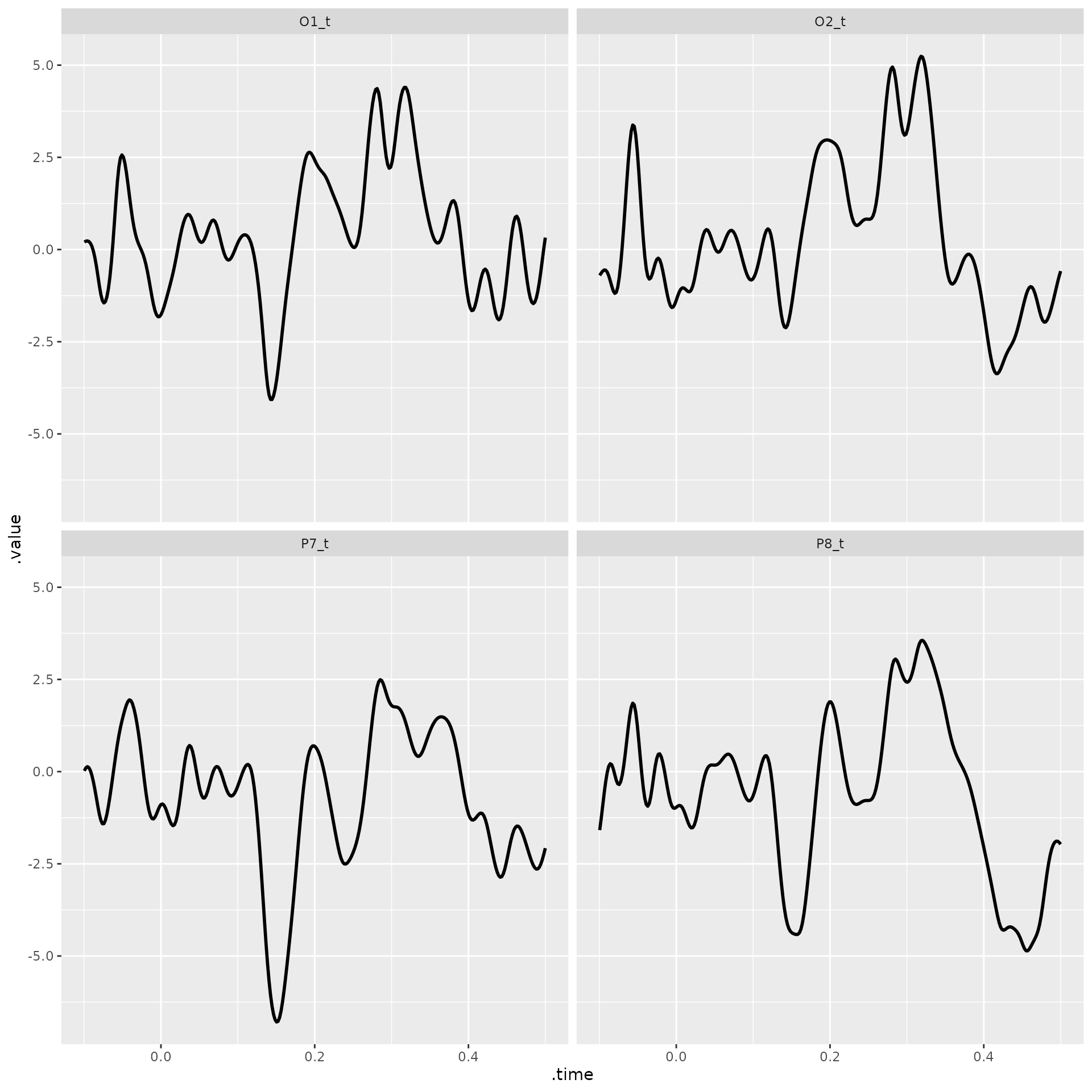
#> 200: 200 s1_faces.vhdr 200 s71 non-facesWith some ggplot skills, we can create customized plots.
ggplot is overloaded to work on an eeg_lst by
first downsampling the signal when necessary, and converting it to a
long-format data frame that is feed into ggplot. This
object can then be customized. (Notice that the channels, or component
names are in a .key column and their amplitude in
.value column, and instead of samples there are now
.time in seconds).
## ggplot uses internally a table that looks like this:
faces_seg |> eeg_filter(.id %in% 1:3) |>
as.data.frame()
#> .time .id .key .value .recording segment description
#> 1 -0.099609375 1 Fp1 -2.239737e-01 s1_faces.vhdr 1 s71
#> 2 -0.097656250 1 Fp1 9.975430e-01 s1_faces.vhdr 1 s71
#> 3 -0.095703125 1 Fp1 2.247707e+00 s1_faces.vhdr 1 s71
#> 4 -0.093750000 1 Fp1 3.336120e+00 s1_faces.vhdr 1 s71
#> 5 -0.091796875 1 Fp1 4.095001e+00 s1_faces.vhdr 1 s71
#> 6 -0.089843750 1 Fp1 4.400744e+00 s1_faces.vhdr 1 s71
#> 7 -0.087890625 1 Fp1 4.192899e+00 s1_faces.vhdr 1 s71
#> 8 -0.085937500 1 Fp1 3.485753e+00 s1_faces.vhdr 1 s71
#> 9 -0.083984375 1 Fp1 2.363034e+00 s1_faces.vhdr 1 s71
#> 10 -0.082031250 1 Fp1 9.716509e-01 s1_faces.vhdr 1 s71
#> 11 -0.080078125 1 Fp1 -4.962482e-01 s1_faces.vhdr 1 s71
#> 12 -0.078125000 1 Fp1 -1.834283e+00 s1_faces.vhdr 1 s71
#> 13 -0.076171875 1 Fp1 -2.845186e+00 s1_faces.vhdr 1 s71
#> 14 -0.074218750 1 Fp1 -3.371554e+00 s1_faces.vhdr 1 s71
#> 15 -0.072265625 1 Fp1 -3.315711e+00 s1_faces.vhdr 1 s71
#> 16 -0.070312500 1 Fp1 -2.656428e+00 s1_faces.vhdr 1 s71
#> 17 -0.068359375 1 Fp1 -1.451257e+00 s1_faces.vhdr 1 s71
#> 18 -0.066406250 1 Fp1 1.668775e-01 s1_faces.vhdr 1 s71
#> 19 -0.064453125 1 Fp1 2.004428e+00 s1_faces.vhdr 1 s71
#> 20 -0.062500000 1 Fp1 3.833147e+00 s1_faces.vhdr 1 s71
#> 21 -0.060546875 1 Fp1 5.417939e+00 s1_faces.vhdr 1 s71
#> 22 -0.058593750 1 Fp1 6.547901e+00 s1_faces.vhdr 1 s71
#> 23 -0.056640625 1 Fp1 7.064995e+00 s1_faces.vhdr 1 s71
#> 24 -0.054687500 1 Fp1 6.887239e+00 s1_faces.vhdr 1 s71
#> 25 -0.052734375 1 Fp1 6.017470e+00 s1_faces.vhdr 1 s71
#> 26 -0.050781250 1 Fp1 4.543313e+00 s1_faces.vhdr 1 s71
#> 27 -0.048828125 1 Fp1 2.630377e+00 s1_faces.vhdr 1 s71
#> 28 -0.046875000 1 Fp1 4.988547e-01 s1_faces.vhdr 1 s71
#> 29 -0.044921875 1 Fp1 -1.604385e+00 s1_faces.vhdr 1 s71
#> 30 -0.042968750 1 Fp1 -3.438169e+00 s1_faces.vhdr 1 s71
#> 31 -0.041015625 1 Fp1 -4.797347e+00 s1_faces.vhdr 1 s71
#> 32 -0.039062500 1 Fp1 -5.540746e+00 s1_faces.vhdr 1 s71
#> 33 -0.037109375 1 Fp1 -5.601511e+00 s1_faces.vhdr 1 s71
#> 34 -0.035156250 1 Fp1 -4.997398e+00 s1_faces.vhdr 1 s71
#> 35 -0.033203125 1 Fp1 -3.831552e+00 s1_faces.vhdr 1 s71
#> 36 -0.031250000 1 Fp1 -2.274974e+00 s1_faces.vhdr 1 s71
#> 37 -0.029296875 1 Fp1 -5.448608e-01 s1_faces.vhdr 1 s71
#> 38 -0.027343750 1 Fp1 1.121354e+00 s1_faces.vhdr 1 s71
#> 39 -0.025390625 1 Fp1 2.496943e+00 s1_faces.vhdr 1 s71
#> 40 -0.023437500 1 Fp1 3.396745e+00 s1_faces.vhdr 1 s71
#> 41 -0.021484375 1 Fp1 3.696361e+00 s1_faces.vhdr 1 s71
#> 42 -0.019531250 1 Fp1 3.344069e+00 s1_faces.vhdr 1 s71
#> 43 -0.017578125 1 Fp1 2.368859e+00 s1_faces.vhdr 1 s71
#> 44 -0.015625000 1 Fp1 8.767626e-01 s1_faces.vhdr 1 s71
#> 45 -0.013671875 1 Fp1 -9.682681e-01 s1_faces.vhdr 1 s71
#> 46 -0.011718750 1 Fp1 -2.963041e+00 s1_faces.vhdr 1 s71
#> 47 -0.009765625 1 Fp1 -4.891834e+00 s1_faces.vhdr 1 s71
#> 48 -0.007812500 1 Fp1 -6.551176e+00 s1_faces.vhdr 1 s71
#> 49 -0.005859375 1 Fp1 -7.777675e+00 s1_faces.vhdr 1 s71
#> 50 -0.003906250 1 Fp1 -8.463097e+00 s1_faces.vhdr 1 s71
#> 51 -0.001953125 1 Fp1 -8.563411e+00 s1_faces.vhdr 1 s71
#> 52 0.000000000 1 Fp1 -8.103625e+00 s1_faces.vhdr 1 s71
#> 53 0.001953125 1 Fp1 -7.167468e+00 s1_faces.vhdr 1 s71
#> 54 0.003906250 1 Fp1 -5.886210e+00 s1_faces.vhdr 1 s71
#> 55 0.005859375 1 Fp1 -4.418849e+00 s1_faces.vhdr 1 s71
#> 56 0.007812500 1 Fp1 -2.933639e+00 s1_faces.vhdr 1 s71
#> 57 0.009765625 1 Fp1 -1.583757e+00 s1_faces.vhdr 1 s71
#> 58 0.011718750 1 Fp1 -4.903709e-01 s1_faces.vhdr 1 s71
#> 59 0.013671875 1 Fp1 2.697942e-01 s1_faces.vhdr 1 s71
#> 60 0.015625000 1 Fp1 6.655293e-01 s1_faces.vhdr 1 s71
#> 61 0.017578125 1 Fp1 7.132909e-01 s1_faces.vhdr 1 s71
#> 62 0.019531250 1 Fp1 4.666661e-01 s1_faces.vhdr 1 s71
#> 63 0.021484375 1 Fp1 3.482913e-03 s1_faces.vhdr 1 s71
#> 64 0.023437500 1 Fp1 -5.829806e-01 s1_faces.vhdr 1 s71
#> 65 0.025390625 1 Fp1 -1.202564e+00 s1_faces.vhdr 1 s71
#> 66 0.027343750 1 Fp1 -1.782230e+00 s1_faces.vhdr 1 s71
#> 67 0.029296875 1 Fp1 -2.274217e+00 s1_faces.vhdr 1 s71
#> 68 0.031250000 1 Fp1 -2.660734e+00 s1_faces.vhdr 1 s71
#> 69 0.033203125 1 Fp1 -2.955666e+00 s1_faces.vhdr 1 s71
#> 70 0.035156250 1 Fp1 -3.206789e+00 s1_faces.vhdr 1 s71
#> 71 0.037109375 1 Fp1 -3.479598e+00 s1_faces.vhdr 1 s71
#> 72 0.039062500 1 Fp1 -3.849415e+00 s1_faces.vhdr 1 s71
#> 73 0.041015625 1 Fp1 -4.388278e+00 s1_faces.vhdr 1 s71
#> 74 0.042968750 1 Fp1 -5.155000e+00 s1_faces.vhdr 1 s71
#> 75 0.044921875 1 Fp1 -6.180153e+00 s1_faces.vhdr 1 s71
#> 76 0.046875000 1 Fp1 -7.462170e+00 s1_faces.vhdr 1 s71
#> 77 0.048828125 1 Fp1 -8.964286e+00 s1_faces.vhdr 1 s71
#> 78 0.050781250 1 Fp1 -1.061373e+01 s1_faces.vhdr 1 s71
#> 79 0.052734375 1 Fp1 -1.231329e+01 s1_faces.vhdr 1 s71
#> 80 0.054687500 1 Fp1 -1.395243e+01 s1_faces.vhdr 1 s71
#> 81 0.056640625 1 Fp1 -1.541582e+01 s1_faces.vhdr 1 s71
#> 82 0.058593750 1 Fp1 -1.659579e+01 s1_faces.vhdr 1 s71
#> 83 0.060546875 1 Fp1 -1.740924e+01 s1_faces.vhdr 1 s71
#> 84 0.062500000 1 Fp1 -1.780176e+01 s1_faces.vhdr 1 s71
#> 85 0.064453125 1 Fp1 -1.775068e+01 s1_faces.vhdr 1 s71
#> 86 0.066406250 1 Fp1 -1.727219e+01 s1_faces.vhdr 1 s71
#> 87 0.068359375 1 Fp1 -1.641756e+01 s1_faces.vhdr 1 s71
#> 88 0.070312500 1 Fp1 -1.526689e+01 s1_faces.vhdr 1 s71
#> 89 0.072265625 1 Fp1 -1.392209e+01 s1_faces.vhdr 1 s71
#> 90 0.074218750 1 Fp1 -1.249775e+01 s1_faces.vhdr 1 s71
#> 91 0.076171875 1 Fp1 -1.111069e+01 s1_faces.vhdr 1 s71
#> 92 0.078125000 1 Fp1 -9.866539e+00 s1_faces.vhdr 1 s71
#> 93 0.080078125 1 Fp1 -8.847984e+00 s1_faces.vhdr 1 s71
#> 94 0.082031250 1 Fp1 -8.106581e+00 s1_faces.vhdr 1 s71
#> 95 0.083984375 1 Fp1 -7.662240e+00 s1_faces.vhdr 1 s71
#> 96 0.085937500 1 Fp1 -7.498032e+00 s1_faces.vhdr 1 s71
#> 97 0.087890625 1 Fp1 -7.562438e+00 s1_faces.vhdr 1 s71
#> 98 0.089843750 1 Fp1 -7.778223e+00 s1_faces.vhdr 1 s71
#> 99 0.091796875 1 Fp1 -8.050479e+00 s1_faces.vhdr 1 s71
#> 100 0.093750000 1 Fp1 -8.279497e+00 s1_faces.vhdr 1 s71
#> 101 0.095703125 1 Fp1 -8.373052e+00 s1_faces.vhdr 1 s71
#> 102 0.097656250 1 Fp1 -8.256166e+00 s1_faces.vhdr 1 s71
#> 103 0.099609375 1 Fp1 -7.881939e+00 s1_faces.vhdr 1 s71
#> 104 0.101562500 1 Fp1 -7.236477e+00 s1_faces.vhdr 1 s71
#> 105 0.103515625 1 Fp1 -6.344185e+00 s1_faces.vhdr 1 s71
#> 106 0.105468750 1 Fp1 -5.262266e+00 s1_faces.vhdr 1 s71
#> 107 0.107421875 1 Fp1 -4.078485e+00 s1_faces.vhdr 1 s71
#> 108 0.109375000 1 Fp1 -2.898918e+00 s1_faces.vhdr 1 s71
#> 109 0.111328125 1 Fp1 -1.834705e+00 s1_faces.vhdr 1 s71
#> 110 0.113281250 1 Fp1 -9.913051e-01 s1_faces.vhdr 1 s71
#> 111 0.115234375 1 Fp1 -4.543431e-01 s1_faces.vhdr 1 s71
#> 112 0.117187500 1 Fp1 -2.808172e-01 s1_faces.vhdr 1 s71
#> 113 0.119140625 1 Fp1 -4.903634e-01 s1_faces.vhdr 1 s71
#> 114 0.121093750 1 Fp1 -1.064283e+00 s1_faces.vhdr 1 s71
#> 115 0.123046875 1 Fp1 -1.943668e+00 s1_faces.vhdr 1 s71
#> 116 0.125000000 1 Fp1 -3.035234e+00 s1_faces.vhdr 1 s71
#> 117 0.126953125 1 Fp1 -4.223626e+00 s1_faces.vhdr 1 s71
#> 118 0.128906250 1 Fp1 -5.382128e+00 s1_faces.vhdr 1 s71
#> 119 0.130859375 1 Fp1 -6.386529e+00 s1_faces.vhdr 1 s71
#> 120 0.132812500 1 Fp1 -7.129893e+00 s1_faces.vhdr 1 s71
#> 121 0.134765625 1 Fp1 -7.537805e+00 s1_faces.vhdr 1 s71
#> 122 0.136718750 1 Fp1 -7.571268e+00 s1_faces.vhdr 1 s71
#> 123 0.138671875 1 Fp1 -7.233492e+00 s1_faces.vhdr 1 s71
#> 124 0.140625000 1 Fp1 -6.569548e+00 s1_faces.vhdr 1 s71
#> 125 0.142578125 1 Fp1 -5.660641e+00 s1_faces.vhdr 1 s71
#> 126 0.144531250 1 Fp1 -4.609919e+00 s1_faces.vhdr 1 s71
#> 127 0.146484375 1 Fp1 -3.528994e+00 s1_faces.vhdr 1 s71
#> 128 0.148437500 1 Fp1 -2.528830e+00 s1_faces.vhdr 1 s71
#> 129 0.150390625 1 Fp1 -1.701509e+00 s1_faces.vhdr 1 s71
#> 130 0.152343750 1 Fp1 -1.113070e+00 s1_faces.vhdr 1 s71
#> 131 0.154296875 1 Fp1 -7.960041e-01 s1_faces.vhdr 1 s71
#> 132 0.156250000 1 Fp1 -7.525606e-01 s1_faces.vhdr 1 s71
#> 133 0.158203125 1 Fp1 -9.551456e-01 s1_faces.vhdr 1 s71
#> 134 0.160156250 1 Fp1 -1.350756e+00 s1_faces.vhdr 1 s71
#> 135 0.162109375 1 Fp1 -1.873586e+00 s1_faces.vhdr 1 s71
#> 136 0.164062500 1 Fp1 -2.451353e+00 s1_faces.vhdr 1 s71
#> 137 0.166015625 1 Fp1 -3.018084e+00 s1_faces.vhdr 1 s71
#> 138 0.167968750 1 Fp1 -3.518105e+00 s1_faces.vhdr 1 s71
#> 139 0.169921875 1 Fp1 -3.915032e+00 s1_faces.vhdr 1 s71
#> 140 0.171875000 1 Fp1 -4.196219e+00 s1_faces.vhdr 1 s71
#> 141 0.173828125 1 Fp1 -4.366605e+00 s1_faces.vhdr 1 s71
#> 142 0.175781250 1 Fp1 -4.449582e+00 s1_faces.vhdr 1 s71
#> 143 0.177734375 1 Fp1 -4.479534e+00 s1_faces.vhdr 1 s71
#> 144 0.179687500 1 Fp1 -4.495663e+00 s1_faces.vhdr 1 s71
#> 145 0.181640625 1 Fp1 -4.538470e+00 s1_faces.vhdr 1 s71
#> 146 0.183593750 1 Fp1 -4.639166e+00 s1_faces.vhdr 1 s71
#> 147 0.185546875 1 Fp1 -4.814374e+00 s1_faces.vhdr 1 s71
#> 148 0.187500000 1 Fp1 -5.068134e+00 s1_faces.vhdr 1 s71
#> 149 0.189453125 1 Fp1 -5.392914e+00 s1_faces.vhdr 1 s71
#> 150 0.191406250 1 Fp1 -5.771779e+00 s1_faces.vhdr 1 s71
#> 151 0.193359375 1 Fp1 -6.185828e+00 s1_faces.vhdr 1 s71
#> 152 0.195312500 1 Fp1 -6.619060e+00 s1_faces.vhdr 1 s71
#> 153 0.197265625 1 Fp1 -7.065608e+00 s1_faces.vhdr 1 s71
#> 154 0.199218750 1 Fp1 -7.528898e+00 s1_faces.vhdr 1 s71
#> 155 0.201171875 1 Fp1 -8.026002e+00 s1_faces.vhdr 1 s71
#> 156 0.203125000 1 Fp1 -8.583017e+00 s1_faces.vhdr 1 s71
#> 157 0.205078125 1 Fp1 -9.233471e+00 s1_faces.vhdr 1 s71
#> 158 0.207031250 1 Fp1 -1.001054e+01 s1_faces.vhdr 1 s71
#> 159 0.208984375 1 Fp1 -1.094285e+01 s1_faces.vhdr 1 s71
#> 160 0.210937500 1 Fp1 -1.204510e+01 s1_faces.vhdr 1 s71
#> 161 0.212890625 1 Fp1 -1.331491e+01 s1_faces.vhdr 1 s71
#> 162 0.214843750 1 Fp1 -1.472885e+01 s1_faces.vhdr 1 s71
#> 163 0.216796875 1 Fp1 -1.624335e+01 s1_faces.vhdr 1 s71
#> 164 0.218750000 1 Fp1 -1.779715e+01 s1_faces.vhdr 1 s71
#> 165 0.220703125 1 Fp1 -1.931900e+01 s1_faces.vhdr 1 s71
#> 166 0.222656250 1 Fp1 -2.073216e+01 s1_faces.vhdr 1 s71
#> 167 0.224609375 1 Fp1 -2.196391e+01 s1_faces.vhdr 1 s71
#> 168 0.226562500 1 Fp1 -2.295457e+01 s1_faces.vhdr 1 s71
#> 169 0.228515625 1 Fp1 -2.366447e+01 s1_faces.vhdr 1 s71
#> 170 0.230468750 1 Fp1 -2.407628e+01 s1_faces.vhdr 1 s71
#> 171 0.232421875 1 Fp1 -2.419777e+01 s1_faces.vhdr 1 s71
#> 172 0.234375000 1 Fp1 -2.405864e+01 s1_faces.vhdr 1 s71
#> 173 0.236328125 1 Fp1 -2.371173e+01 s1_faces.vhdr 1 s71
#> 174 0.238281250 1 Fp1 -2.322517e+01 s1_faces.vhdr 1 s71
#> 175 0.240234375 1 Fp1 -2.267266e+01 s1_faces.vhdr 1 s71
#> 176 0.242187500 1 Fp1 -2.212478e+01 s1_faces.vhdr 1 s71
#> 177 0.244140625 1 Fp1 -2.164063e+01 s1_faces.vhdr 1 s71
#> 178 0.246093750 1 Fp1 -2.126114e+01 s1_faces.vhdr 1 s71
#> 179 0.248046875 1 Fp1 -2.100552e+01 s1_faces.vhdr 1 s71
#> 180 0.250000000 1 Fp1 -2.087226e+01 s1_faces.vhdr 1 s71
#> 181 0.251953125 1 Fp1 -2.083915e+01 s1_faces.vhdr 1 s71
#> 182 0.253906250 1 Fp1 -2.086801e+01 s1_faces.vhdr 1 s71
#> 183 0.255859375 1 Fp1 -2.091545e+01 s1_faces.vhdr 1 s71
#> 184 0.257812500 1 Fp1 -2.093737e+01 s1_faces.vhdr 1 s71
#> 185 0.259765625 1 Fp1 -2.089675e+01 s1_faces.vhdr 1 s71
#> 186 0.261718750 1 Fp1 -2.076796e+01 s1_faces.vhdr 1 s71
#> 187 0.263671875 1 Fp1 -2.054024e+01 s1_faces.vhdr 1 s71
#> 188 0.265625000 1 Fp1 -2.022135e+01 s1_faces.vhdr 1 s71
#> 189 0.267578125 1 Fp1 -1.983543e+01 s1_faces.vhdr 1 s71
#> 190 0.269531250 1 Fp1 -1.941927e+01 s1_faces.vhdr 1 s71
#> 191 0.271484375 1 Fp1 -1.901655e+01 s1_faces.vhdr 1 s71
#> 192 0.273437500 1 Fp1 -1.867090e+01 s1_faces.vhdr 1 s71
#> 193 0.275390625 1 Fp1 -1.842160e+01 s1_faces.vhdr 1 s71
#> 194 0.277343750 1 Fp1 -1.829740e+01 s1_faces.vhdr 1 s71
#> 195 0.279296875 1 Fp1 -1.831317e+01 s1_faces.vhdr 1 s71
#> 196 0.281250000 1 Fp1 -1.846551e+01 s1_faces.vhdr 1 s71
#> 197 0.283203125 1 Fp1 -1.873093e+01 s1_faces.vhdr 1 s71
#> 198 0.285156250 1 Fp1 -1.906924e+01 s1_faces.vhdr 1 s71
#> 199 0.287109375 1 Fp1 -1.942763e+01 s1_faces.vhdr 1 s71
#> 200 0.289062500 1 Fp1 -1.974295e+01 s1_faces.vhdr 1 s71
#> 201 0.291015625 1 Fp1 -1.994861e+01 s1_faces.vhdr 1 s71
#> 202 0.292968750 1 Fp1 -1.998190e+01 s1_faces.vhdr 1 s71
#> 203 0.294921875 1 Fp1 -1.979184e+01 s1_faces.vhdr 1 s71
#> 204 0.296875000 1 Fp1 -1.934498e+01 s1_faces.vhdr 1 s71
#> 205 0.298828125 1 Fp1 -1.862693e+01 s1_faces.vhdr 1 s71
#> 206 0.300781250 1 Fp1 -1.764578e+01 s1_faces.vhdr 1 s71
#> 207 0.302734375 1 Fp1 -1.642952e+01 s1_faces.vhdr 1 s71
#> 208 0.304687500 1 Fp1 -1.502425e+01 s1_faces.vhdr 1 s71
#> 209 0.306640625 1 Fp1 -1.348922e+01 s1_faces.vhdr 1 s71
#> 210 0.308593750 1 Fp1 -1.189333e+01 s1_faces.vhdr 1 s71
#> 211 0.310546875 1 Fp1 -1.030801e+01 s1_faces.vhdr 1 s71
#> 212 0.312500000 1 Fp1 -8.802739e+00 s1_faces.vhdr 1 s71
#> 213 0.314453125 1 Fp1 -7.444267e+00 s1_faces.vhdr 1 s71
#> 214 0.316406250 1 Fp1 -6.288834e+00 s1_faces.vhdr 1 s71
#> 215 0.318359375 1 Fp1 -5.380901e+00 s1_faces.vhdr 1 s71
#> 216 0.320312500 1 Fp1 -4.748934e+00 s1_faces.vhdr 1 s71
#> 217 0.322265625 1 Fp1 -4.410985e+00 s1_faces.vhdr 1 s71
#> 218 0.324218750 1 Fp1 -4.371350e+00 s1_faces.vhdr 1 s71
#> 219 0.326171875 1 Fp1 -4.618921e+00 s1_faces.vhdr 1 s71
#> 220 0.328125000 1 Fp1 -5.131633e+00 s1_faces.vhdr 1 s71
#> 221 0.330078125 1 Fp1 -5.877832e+00 s1_faces.vhdr 1 s71
#> 222 0.332031250 1 Fp1 -6.817069e+00 s1_faces.vhdr 1 s71
#> 223 0.333984375 1 Fp1 -7.904834e+00 s1_faces.vhdr 1 s71
#> 224 0.335937500 1 Fp1 -9.091014e+00 s1_faces.vhdr 1 s71
#> 225 0.337890625 1 Fp1 -1.032183e+01 s1_faces.vhdr 1 s71
#> 226 0.339843750 1 Fp1 -1.154264e+01 s1_faces.vhdr 1 s71
#> 227 0.341796875 1 Fp1 -1.270008e+01 s1_faces.vhdr 1 s71
#> 228 0.343750000 1 Fp1 -1.374167e+01 s1_faces.vhdr 1 s71
#> 229 0.345703125 1 Fp1 -1.462177e+01 s1_faces.vhdr 1 s71
#> 230 0.347656250 1 Fp1 -1.530042e+01 s1_faces.vhdr 1 s71
#> 231 0.349609375 1 Fp1 -1.574794e+01 s1_faces.vhdr 1 s71
#> 232 0.351562500 1 Fp1 -1.594455e+01 s1_faces.vhdr 1 s71
#> 233 0.353515625 1 Fp1 -1.588357e+01 s1_faces.vhdr 1 s71
#> 234 0.355468750 1 Fp1 -1.557544e+01 s1_faces.vhdr 1 s71
#> 235 0.357421875 1 Fp1 -1.504653e+01 s1_faces.vhdr 1 s71
#> 236 0.359375000 1 Fp1 -1.433758e+01 s1_faces.vhdr 1 s71
#> 237 0.361328125 1 Fp1 -1.350057e+01 s1_faces.vhdr 1 s71
#> 238 0.363281250 1 Fp1 -1.259849e+01 s1_faces.vhdr 1 s71
#> 239 0.365234375 1 Fp1 -1.169646e+01 s1_faces.vhdr 1 s71
#> 240 0.367187500 1 Fp1 -1.085513e+01 s1_faces.vhdr 1 s71
#> 241 0.369140625 1 Fp1 -1.013026e+01 s1_faces.vhdr 1 s71
#> 242 0.371093750 1 Fp1 -9.566449e+00 s1_faces.vhdr 1 s71
#> 243 0.373046875 1 Fp1 -9.194910e+00 s1_faces.vhdr 1 s71
#> 244 0.375000000 1 Fp1 -9.030689e+00 s1_faces.vhdr 1 s71
#> 245 0.376953125 1 Fp1 -9.074888e+00 s1_faces.vhdr 1 s71
#> 246 0.378906250 1 Fp1 -9.315735e+00 s1_faces.vhdr 1 s71
#> 247 0.380859375 1 Fp1 -9.729150e+00 s1_faces.vhdr 1 s71
#> 248 0.382812500 1 Fp1 -1.028387e+01 s1_faces.vhdr 1 s71
#> 249 0.384765625 1 Fp1 -1.094235e+01 s1_faces.vhdr 1 s71
#> 250 0.386718750 1 Fp1 -1.166538e+01 s1_faces.vhdr 1 s71
#> 251 0.388671875 1 Fp1 -1.241576e+01 s1_faces.vhdr 1 s71
#> 252 0.390625000 1 Fp1 -1.315699e+01 s1_faces.vhdr 1 s71
#> 253 0.392578125 1 Fp1 -1.385454e+01 s1_faces.vhdr 1 s71
#> 254 0.394531250 1 Fp1 -1.447556e+01 s1_faces.vhdr 1 s71
#> 255 0.396484375 1 Fp1 -1.498754e+01 s1_faces.vhdr 1 s71
#> 256 0.398437500 1 Fp1 -1.536032e+01 s1_faces.vhdr 1 s71
#> 257 0.400390625 1 Fp1 -1.556841e+01 s1_faces.vhdr 1 s71
#> 258 0.402343750 1 Fp1 -1.559108e+01 s1_faces.vhdr 1 s71
#> 259 0.404296875 1 Fp1 -1.541074e+01 s1_faces.vhdr 1 s71
#> 260 0.406250000 1 Fp1 -1.501630e+01 s1_faces.vhdr 1 s71
#> 261 0.408203125 1 Fp1 -1.440797e+01 s1_faces.vhdr 1 s71
#> 262 0.410156250 1 Fp1 -1.360080e+01 s1_faces.vhdr 1 s71
#> 263 0.412109375 1 Fp1 -1.262585e+01 s1_faces.vhdr 1 s71
#> 264 0.414062500 1 Fp1 -1.153561e+01 s1_faces.vhdr 1 s71
#> 265 0.416015625 1 Fp1 -1.040013e+01 s1_faces.vhdr 1 s71
#> 266 0.417968750 1 Fp1 -9.303312e+00 s1_faces.vhdr 1 s71
#> 267 0.419921875 1 Fp1 -8.334693e+00 s1_faces.vhdr 1 s71
#> 268 0.421875000 1 Fp1 -7.583176e+00 s1_faces.vhdr 1 s71
#> 269 0.423828125 1 Fp1 -7.128139e+00 s1_faces.vhdr 1 s71
#> 270 0.425781250 1 Fp1 -7.021208e+00 s1_faces.vhdr 1 s71
#> 271 0.427734375 1 Fp1 -7.284902e+00 s1_faces.vhdr 1 s71
#> 272 0.429687500 1 Fp1 -7.905391e+00 s1_faces.vhdr 1 s71
#> 273 0.431640625 1 Fp1 -8.829486e+00 s1_faces.vhdr 1 s71
#> 274 0.433593750 1 Fp1 -9.967917e+00 s1_faces.vhdr 1 s71
#> 275 0.435546875 1 Fp1 -1.120659e+01 s1_faces.vhdr 1 s71
#> 276 0.437500000 1 Fp1 -1.241608e+01 s1_faces.vhdr 1 s71
#> 277 0.439453125 1 Fp1 -1.346629e+01 s1_faces.vhdr 1 s71
#> 278 0.441406250 1 Fp1 -1.424178e+01 s1_faces.vhdr 1 s71
#> 279 0.443359375 1 Fp1 -1.465293e+01 s1_faces.vhdr 1 s71
#> 280 0.445312500 1 Fp1 -1.464758e+01 s1_faces.vhdr 1 s71
#> 281 0.447265625 1 Fp1 -1.421542e+01 s1_faces.vhdr 1 s71
#> 282 0.449218750 1 Fp1 -1.339040e+01 s1_faces.vhdr 1 s71
#> 283 0.451171875 1 Fp1 -1.224514e+01 s1_faces.vhdr 1 s71
#> 284 0.453125000 1 Fp1 -1.087902e+01 s1_faces.vhdr 1 s71
#> 285 0.455078125 1 Fp1 -9.406730e+00 s1_faces.vhdr 1 s71
#> 286 0.457031250 1 Fp1 -7.943253e+00 s1_faces.vhdr 1 s71
#> 287 0.458984375 1 Fp1 -6.588981e+00 s1_faces.vhdr 1 s71
#> 288 0.460937500 1 Fp1 -5.416370e+00 s1_faces.vhdr 1 s71
#> 289 0.462890625 1 Fp1 -4.464978e+00 s1_faces.vhdr 1 s71
#> 290 0.464843750 1 Fp1 -3.737533e+00 s1_faces.vhdr 1 s71
#> 291 0.466796875 1 Fp1 -3.206004e+00 s1_faces.vhdr 1 s71
#> 292 0.468750000 1 Fp1 -2.820421e+00 s1_faces.vhdr 1 s71
#> 293 0.470703125 1 Fp1 -2.520905e+00 s1_faces.vhdr 1 s71
#> 294 0.472656250 1 Fp1 -2.249321e+00 s1_faces.vhdr 1 s71
#> 295 0.474609375 1 Fp1 -1.963662e+00 s1_faces.vhdr 1 s71
#> 296 0.476562500 1 Fp1 -1.652082e+00 s1_faces.vhdr 1 s71
#> 297 0.478515625 1 Fp1 -1.334791e+00 s1_faces.vhdr 1 s71
#> 298 0.480468750 1 Fp1 -1.062855e+00 s1_faces.vhdr 1 s71
#> 299 0.482421875 1 Fp1 -9.072799e-01 s1_faces.vhdr 1 s71
#> 300 0.484375000 1 Fp1 -9.498670e-01 s1_faces.vhdr 1 s71
#> 301 0.486328125 1 Fp1 -1.265373e+00 s1_faces.vhdr 1 s71
#> 302 0.488281250 1 Fp1 -1.904152e+00 s1_faces.vhdr 1 s71
#> 303 0.490234375 1 Fp1 -2.879418e+00 s1_faces.vhdr 1 s71
#> 304 0.492187500 1 Fp1 -4.156086e+00 s1_faces.vhdr 1 s71
#> 305 0.494140625 1 Fp1 -5.651537e+00 s1_faces.vhdr 1 s71
#> 306 0.496093750 1 Fp1 -7.240843e+00 s1_faces.vhdr 1 s71
#> 307 0.498046875 1 Fp1 -8.768753e+00 s1_faces.vhdr 1 s71
#> 308 0.500000000 1 Fp1 -1.006624e+01 s1_faces.vhdr 1 s71
#> 309 -0.099609375 2 Fp1 -2.943005e+00 s1_faces.vhdr 2 s71
#> 310 -0.097656250 2 Fp1 -2.918656e+00 s1_faces.vhdr 2 s71
#> 311 -0.095703125 2 Fp1 -2.600848e+00 s1_faces.vhdr 2 s71
#> 312 -0.093750000 2 Fp1 -2.017334e+00 s1_faces.vhdr 2 s71
#> 313 -0.091796875 2 Fp1 -1.216420e+00 s1_faces.vhdr 2 s71
#> 314 -0.089843750 2 Fp1 -2.607514e-01 s1_faces.vhdr 2 s71
#> 315 -0.087890625 2 Fp1 7.812880e-01 s1_faces.vhdr 2 s71
#> 316 -0.085937500 2 Fp1 1.838766e+00 s1_faces.vhdr 2 s71
#> 317 -0.083984375 2 Fp1 2.842397e+00 s1_faces.vhdr 2 s71
#> 318 -0.082031250 2 Fp1 3.733779e+00 s1_faces.vhdr 2 s71
#> 319 -0.080078125 2 Fp1 4.467685e+00 s1_faces.vhdr 2 s71
#> 320 -0.078125000 2 Fp1 5.013888e+00 s1_faces.vhdr 2 s71
#> 321 -0.076171875 2 Fp1 5.360589e+00 s1_faces.vhdr 2 s71
#> 322 -0.074218750 2 Fp1 5.511626e+00 s1_faces.vhdr 2 s71
#> 323 -0.072265625 2 Fp1 5.483234e+00 s1_faces.vhdr 2 s71
#> 324 -0.070312500 2 Fp1 5.300074e+00 s1_faces.vhdr 2 s71
#> 325 -0.068359375 2 Fp1 4.989354e+00 s1_faces.vhdr 2 s71
#> 326 -0.066406250 2 Fp1 4.578799e+00 s1_faces.vhdr 2 s71
#> 327 -0.064453125 2 Fp1 4.092726e+00 s1_faces.vhdr 2 s71
#> 328 -0.062500000 2 Fp1 3.552177e+00 s1_faces.vhdr 2 s71
#> 329 -0.060546875 2 Fp1 2.971738e+00 s1_faces.vhdr 2 s71
#> 330 -0.058593750 2 Fp1 2.361256e+00 s1_faces.vhdr 2 s71
#> 331 -0.056640625 2 Fp1 1.726422e+00 s1_faces.vhdr 2 s71
#> 332 -0.054687500 2 Fp1 1.074176e+00 s1_faces.vhdr 2 s71
#> 333 -0.052734375 2 Fp1 4.103475e-01 s1_faces.vhdr 2 s71
#> 334 -0.050781250 2 Fp1 -2.535241e-01 s1_faces.vhdr 2 s71
#> 335 -0.048828125 2 Fp1 -9.042469e-01 s1_faces.vhdr 2 s71
#> 336 -0.046875000 2 Fp1 -1.526534e+00 s1_faces.vhdr 2 s71
#> 337 -0.044921875 2 Fp1 -2.099639e+00 s1_faces.vhdr 2 s71
#> 338 -0.042968750 2 Fp1 -2.601276e+00 s1_faces.vhdr 2 s71
#> 339 -0.041015625 2 Fp1 -3.010272e+00 s1_faces.vhdr 2 s71
#> 340 -0.039062500 2 Fp1 -3.309701e+00 s1_faces.vhdr 2 s71
#> 341 -0.037109375 2 Fp1 -3.490249e+00 s1_faces.vhdr 2 s71
#> 342 -0.035156250 2 Fp1 -3.551372e+00 s1_faces.vhdr 2 s71
#> 343 -0.033203125 2 Fp1 -3.500877e+00 s1_faces.vhdr 2 s71
#> 344 -0.031250000 2 Fp1 -3.357698e+00 s1_faces.vhdr 2 s71
#> 345 -0.029296875 2 Fp1 -3.147227e+00 s1_faces.vhdr 2 s71
#> 346 -0.027343750 2 Fp1 -2.900897e+00 s1_faces.vhdr 2 s71
#> 347 -0.025390625 2 Fp1 -2.650187e+00 s1_faces.vhdr 2 s71
#> 348 -0.023437500 2 Fp1 -2.420901e+00 s1_faces.vhdr 2 s71
#> 349 -0.021484375 2 Fp1 -2.230008e+00 s1_faces.vhdr 2 s71
#> 350 -0.019531250 2 Fp1 -2.084571e+00 s1_faces.vhdr 2 s71
#> 351 -0.017578125 2 Fp1 -1.975624e+00 s1_faces.vhdr 2 s71
#> 352 -0.015625000 2 Fp1 -1.884147e+00 s1_faces.vhdr 2 s71
#> 353 -0.013671875 2 Fp1 -1.784357e+00 s1_faces.vhdr 2 s71
#> 354 -0.011718750 2 Fp1 -1.649367e+00 s1_faces.vhdr 2 s71
#> 355 -0.009765625 2 Fp1 -1.453378e+00 s1_faces.vhdr 2 s71
#> 356 -0.007812500 2 Fp1 -1.178218e+00 s1_faces.vhdr 2 s71
#> 357 -0.005859375 2 Fp1 -8.226791e-01 s1_faces.vhdr 2 s71
#> 358 -0.003906250 2 Fp1 -4.015053e-01 s1_faces.vhdr 2 s71
#> 359 -0.001953125 2 Fp1 5.515102e-02 s1_faces.vhdr 2 s71
#> 360 0.000000000 2 Fp1 5.009034e-01 s1_faces.vhdr 2 s71
#> 361 0.001953125 2 Fp1 8.794682e-01 s1_faces.vhdr 2 s71
#> 362 0.003906250 2 Fp1 1.130473e+00 s1_faces.vhdr 2 s71
#> 363 0.005859375 2 Fp1 1.195505e+00 s1_faces.vhdr 2 s71
#> 364 0.007812500 2 Fp1 1.026834e+00 s1_faces.vhdr 2 s71
#> 365 0.009765625 2 Fp1 5.934945e-01 s1_faces.vhdr 2 s71
#> 366 0.011718750 2 Fp1 -1.143227e-01 s1_faces.vhdr 2 s71
#> 367 0.013671875 2 Fp1 -1.081430e+00 s1_faces.vhdr 2 s71
#> 368 0.015625000 2 Fp1 -2.268602e+00 s1_faces.vhdr 2 s71
#> 369 0.017578125 2 Fp1 -3.612589e+00 s1_faces.vhdr 2 s71
#> 370 0.019531250 2 Fp1 -5.031717e+00 s1_faces.vhdr 2 s71
#> 371 0.021484375 2 Fp1 -6.434470e+00 s1_faces.vhdr 2 s71
#> 372 0.023437500 2 Fp1 -7.727604e+00 s1_faces.vhdr 2 s71
#> 373 0.025390625 2 Fp1 -8.821715e+00 s1_faces.vhdr 2 s71
#> 374 0.027343750 2 Fp1 -9.643640e+00 s1_faces.vhdr 2 s71
#> 375 0.029296875 2 Fp1 -1.014096e+01 s1_faces.vhdr 2 s71
#> 376 0.031250000 2 Fp1 -1.028625e+01 s1_faces.vhdr 2 s71
#> 377 0.033203125 2 Fp1 -1.007983e+01 s1_faces.vhdr 2 s71
#> 378 0.035156250 2 Fp1 -9.545381e+00 s1_faces.vhdr 2 s71
#> 379 0.037109375 2 Fp1 -8.729963e+00 s1_faces.vhdr 2 s71
#> 380 0.039062500 2 Fp1 -7.697006e+00 s1_faces.vhdr 2 s71
#> 381 0.041015625 2 Fp1 -6.517814e+00 s1_faces.vhdr 2 s71
#> 382 0.042968750 2 Fp1 -5.269487e+00 s1_faces.vhdr 2 s71
#> 383 0.044921875 2 Fp1 -4.027164e+00 s1_faces.vhdr 2 s71
#> 384 0.046875000 2 Fp1 -2.856947e+00 s1_faces.vhdr 2 s71
#> 385 0.048828125 2 Fp1 -1.814868e+00 s1_faces.vhdr 2 s71
#> 386 0.050781250 2 Fp1 -9.464816e-01 s1_faces.vhdr 2 s71
#> 387 0.052734375 2 Fp1 -2.842316e-01 s1_faces.vhdr 2 s71
#> 388 0.054687500 2 Fp1 1.551709e-01 s1_faces.vhdr 2 s71
#> 389 0.056640625 2 Fp1 3.660372e-01 s1_faces.vhdr 2 s71
#> 390 0.058593750 2 Fp1 3.524796e-01 s1_faces.vhdr 2 s71
#> 391 0.060546875 2 Fp1 1.303894e-01 s1_faces.vhdr 2 s71
#> 392 0.062500000 2 Fp1 -2.769612e-01 s1_faces.vhdr 2 s71
#> 393 0.064453125 2 Fp1 -8.375864e-01 s1_faces.vhdr 2 s71
#> 394 0.066406250 2 Fp1 -1.512285e+00 s1_faces.vhdr 2 s71
#> 395 0.068359375 2 Fp1 -2.260522e+00 s1_faces.vhdr 2 s71
#> 396 0.070312500 2 Fp1 -3.035468e+00 s1_faces.vhdr 2 s71
#> 397 0.072265625 2 Fp1 -3.785520e+00 s1_faces.vhdr 2 s71
#> 398 0.074218750 2 Fp1 -4.454396e+00 s1_faces.vhdr 2 s71
#> 399 0.076171875 2 Fp1 -4.984129e+00 s1_faces.vhdr 2 s71
#> 400 0.078125000 2 Fp1 -5.317260e+00 s1_faces.vhdr 2 s71
#> 401 0.080078125 2 Fp1 -5.397915e+00 s1_faces.vhdr 2 s71
#> 402 0.082031250 2 Fp1 -5.175688e+00 s1_faces.vhdr 2 s71
#> 403 0.083984375 2 Fp1 -4.609971e+00 s1_faces.vhdr 2 s71
#> 404 0.085937500 2 Fp1 -3.675856e+00 s1_faces.vhdr 2 s71
#> 405 0.087890625 2 Fp1 -2.369432e+00 s1_faces.vhdr 2 s71
#> 406 0.089843750 2 Fp1 -7.117335e-01 s1_faces.vhdr 2 s71
#> 407 0.091796875 2 Fp1 1.251993e+00 s1_faces.vhdr 2 s71
#> 408 0.093750000 2 Fp1 3.448901e+00 s1_faces.vhdr 2 s71
#> 409 0.095703125 2 Fp1 5.785824e+00 s1_faces.vhdr 2 s71
#> 410 0.097656250 2 Fp1 8.151735e+00 s1_faces.vhdr 2 s71
#> 411 0.099609375 2 Fp1 1.042651e+01 s1_faces.vhdr 2 s71
#> 412 0.101562500 2 Fp1 1.248716e+01 s1_faces.vhdr 2 s71
#> 413 0.103515625 2 Fp1 1.421921e+01 s1_faces.vhdr 2 s71
#> 414 0.105468750 2 Fp1 1.552677e+01 s1_faces.vhdr 2 s71
#> 415 0.107421875 2 Fp1 1.634207e+01 s1_faces.vhdr 2 s71
#> 416 0.109375000 2 Fp1 1.662866e+01 s1_faces.vhdr 2 s71
#> 417 0.111328125 2 Fp1 1.638479e+01 s1_faces.vhdr 2 s71
#> 418 0.113281250 2 Fp1 1.564872e+01 s1_faces.vhdr 2 s71
#> 419 0.115234375 2 Fp1 1.449174e+01 s1_faces.vhdr 2 s71
#> 420 0.117187500 2 Fp1 1.301151e+01 s1_faces.vhdr 2 s71
#> 421 0.119140625 2 Fp1 1.132388e+01 s1_faces.vhdr 2 s71
#> 422 0.121093750 2 Fp1 9.553847e+00 s1_faces.vhdr 2 s71
#> 423 0.123046875 2 Fp1 7.821436e+00 s1_faces.vhdr 2 s71
#> 424 0.125000000 2 Fp1 6.233006e+00 s1_faces.vhdr 2 s71
#> 425 0.126953125 2 Fp1 4.868509e+00 s1_faces.vhdr 2 s71
#> 426 0.128906250 2 Fp1 3.773750e+00 s1_faces.vhdr 2 s71
#> 427 0.130859375 2 Fp1 2.959273e+00 s1_faces.vhdr 2 s71
#> 428 0.132812500 2 Fp1 2.402442e+00 s1_faces.vhdr 2 s71
#> 429 0.134765625 2 Fp1 2.047638e+00 s1_faces.vhdr 2 s71
#> 430 0.136718750 2 Fp1 1.817087e+00 s1_faces.vhdr 2 s71
#> 431 0.138671875 2 Fp1 1.622236e+00 s1_faces.vhdr 2 s71
#> 432 0.140625000 2 Fp1 1.374180e+00 s1_faces.vhdr 2 s71
#> 433 0.142578125 2 Fp1 9.934579e-01 s1_faces.vhdr 2 s71
#> 434 0.144531250 2 Fp1 4.205124e-01 s1_faces.vhdr 2 s71
#> 435 0.146484375 2 Fp1 -3.775397e-01 s1_faces.vhdr 2 s71
#> 436 0.148437500 2 Fp1 -1.404333e+00 s1_faces.vhdr 2 s71
#> 437 0.150390625 2 Fp1 -2.637825e+00 s1_faces.vhdr 2 s71
#> 438 0.152343750 2 Fp1 -4.032993e+00 s1_faces.vhdr 2 s71
#> 439 0.154296875 2 Fp1 -5.526829e+00 s1_faces.vhdr 2 s71
#> 440 0.156250000 2 Fp1 -7.050901e+00 s1_faces.vhdr 2 s71
#> 441 0.158203125 2 Fp1 -8.535493e+00 s1_faces.vhdr 2 s71
#> 442 0.160156250 2 Fp1 -9.916845e+00 s1_faces.vhdr 2 s71
#> 443 0.162109375 2 Fp1 -1.114491e+01 s1_faces.vhdr 2 s71
#> 444 0.164062500 2 Fp1 -1.218625e+01 s1_faces.vhdr 2 s71
#> 445 0.166015625 2 Fp1 -1.302585e+01 s1_faces.vhdr 2 s71
#> 446 0.167968750 2 Fp1 -1.366901e+01 s1_faces.vhdr 2 s71
#> 447 0.169921875 2 Fp1 -1.413590e+01 s1_faces.vhdr 2 s71
#> 448 0.171875000 2 Fp1 -1.445611e+01 s1_faces.vhdr 2 s71
#> 449 0.173828125 2 Fp1 -1.466631e+01 s1_faces.vhdr 2 s71
#> 450 0.175781250 2 Fp1 -1.480333e+01 s1_faces.vhdr 2 s71
#> 451 0.177734375 2 Fp1 -1.489954e+01 s1_faces.vhdr 2 s71
#> 452 0.179687500 2 Fp1 -1.498086e+01 s1_faces.vhdr 2 s71
#> 453 0.181640625 2 Fp1 -1.506335e+01 s1_faces.vhdr 2 s71
#> 454 0.183593750 2 Fp1 -1.515447e+01 s1_faces.vhdr 2 s71
#> 455 0.185546875 2 Fp1 -1.525183e+01 s1_faces.vhdr 2 s71
#> 456 0.187500000 2 Fp1 -1.534773e+01 s1_faces.vhdr 2 s71
#> 457 0.189453125 2 Fp1 -1.543079e+01 s1_faces.vhdr 2 s71
#> 458 0.191406250 2 Fp1 -1.548940e+01 s1_faces.vhdr 2 s71
#> 459 0.193359375 2 Fp1 -1.551074e+01 s1_faces.vhdr 2 s71
#> 460 0.195312500 2 Fp1 -1.548178e+01 s1_faces.vhdr 2 s71
#> 461 0.197265625 2 Fp1 -1.538828e+01 s1_faces.vhdr 2 s71
#> 462 0.199218750 2 Fp1 -1.521666e+01 s1_faces.vhdr 2 s71
#> 463 0.201171875 2 Fp1 -1.495679e+01 s1_faces.vhdr 2 s71
#> 464 0.203125000 2 Fp1 -1.459723e+01 s1_faces.vhdr 2 s71
#> 465 0.205078125 2 Fp1 -1.413300e+01 s1_faces.vhdr 2 s71
#> 466 0.207031250 2 Fp1 -1.356733e+01 s1_faces.vhdr 2 s71
#> 467 0.208984375 2 Fp1 -1.291655e+01 s1_faces.vhdr 2 s71
#> 468 0.210937500 2 Fp1 -1.221391e+01 s1_faces.vhdr 2 s71
#> 469 0.212890625 2 Fp1 -1.150674e+01 s1_faces.vhdr 2 s71
#> 470 0.214843750 2 Fp1 -1.085753e+01 s1_faces.vhdr 2 s71
#> 471 0.216796875 2 Fp1 -1.033877e+01 s1_faces.vhdr 2 s71
#> 472 0.218750000 2 Fp1 -1.002757e+01 s1_faces.vhdr 2 s71
#> 473 0.220703125 2 Fp1 -9.996890e+00 s1_faces.vhdr 2 s71
#> 474 0.222656250 2 Fp1 -1.031127e+01 s1_faces.vhdr 2 s71
#> 475 0.224609375 2 Fp1 -1.101397e+01 s1_faces.vhdr 2 s71
#> 476 0.226562500 2 Fp1 -1.211704e+01 s1_faces.vhdr 2 s71
#> 477 0.228515625 2 Fp1 -1.359939e+01 s1_faces.vhdr 2 s71
#> 478 0.230468750 2 Fp1 -1.540662e+01 s1_faces.vhdr 2 s71
#> 479 0.232421875 2 Fp1 -1.745102e+01 s1_faces.vhdr 2 s71
#> 480 0.234375000 2 Fp1 -1.961797e+01 s1_faces.vhdr 2 s71
#> 481 0.236328125 2 Fp1 -2.177886e+01 s1_faces.vhdr 2 s71
#> 482 0.238281250 2 Fp1 -2.380178e+01 s1_faces.vhdr 2 s71
#> 483 0.240234375 2 Fp1 -2.556532e+01 s1_faces.vhdr 2 s71
#> 484 0.242187500 2 Fp1 -2.697723e+01 s1_faces.vhdr 2 s71
#> 485 0.244140625 2 Fp1 -2.798183e+01 s1_faces.vhdr 2 s71
#> 486 0.246093750 2 Fp1 -2.856510e+01 s1_faces.vhdr 2 s71
#> 487 0.248046875 2 Fp1 -2.876144e+01 s1_faces.vhdr 2 s71
#> 488 0.250000000 2 Fp1 -2.864934e+01 s1_faces.vhdr 2 s71
#> 489 0.251953125 2 Fp1 -2.833740e+01 s1_faces.vhdr 2 s71
#> 490 0.253906250 2 Fp1 -2.795296e+01 s1_faces.vhdr 2 s71
#> 491 0.255859375 2 Fp1 -2.762438e+01 s1_faces.vhdr 2 s71
#> 492 0.257812500 2 Fp1 -2.746074e+01 s1_faces.vhdr 2 s71
#> 493 0.259765625 2 Fp1 -2.754050e+01 s1_faces.vhdr 2 s71
#> 494 0.261718750 2 Fp1 -2.789849e+01 s1_faces.vhdr 2 s71
#> 495 0.263671875 2 Fp1 -2.851901e+01 s1_faces.vhdr 2 s71
#> 496 0.265625000 2 Fp1 -2.933942e+01 s1_faces.vhdr 2 s71
#> 497 0.267578125 2 Fp1 -3.025951e+01 s1_faces.vhdr 2 s71
#> 498 0.269531250 2 Fp1 -3.115401e+01 s1_faces.vhdr 2 s71
#> 499 0.271484375 2 Fp1 -3.189003e+01 s1_faces.vhdr 2 s71
#> 500 0.273437500 2 Fp1 -3.234325e+01 s1_faces.vhdr 2 s71
#> 501 0.275390625 2 Fp1 -3.241655e+01 s1_faces.vhdr 2 s71
#> 502 0.277343750 2 Fp1 -3.205270e+01 s1_faces.vhdr 2 s71
#> 503 0.279296875 2 Fp1 -3.123907e+01 s1_faces.vhdr 2 s71
#> 504 0.281250000 2 Fp1 -3.001236e+01 s1_faces.vhdr 2 s71
#> 505 0.283203125 2 Fp1 -2.844882e+01 s1_faces.vhdr 2 s71
#> 506 0.285156250 2 Fp1 -2.665680e+01 s1_faces.vhdr 2 s71
#> 507 0.287109375 2 Fp1 -2.476428e+01 s1_faces.vhdr 2 s71
#> 508 0.289062500 2 Fp1 -2.290407e+01 s1_faces.vhdr 2 s71
#> 509 0.291015625 2 Fp1 -2.119753e+01 s1_faces.vhdr 2 s71
#> 510 0.292968750 2 Fp1 -1.974173e+01 s1_faces.vhdr 2 s71
#> 511 0.294921875 2 Fp1 -1.859924e+01 s1_faces.vhdr 2 s71
#> 512 0.296875000 2 Fp1 -1.779780e+01 s1_faces.vhdr 2 s71
#> 513 0.298828125 2 Fp1 -1.732985e+01 s1_faces.vhdr 2 s71
#> 514 0.300781250 2 Fp1 -1.715674e+01 s1_faces.vhdr 2 s71
#> 515 0.302734375 2 Fp1 -1.722103e+01 s1_faces.vhdr 2 s71
#> 516 0.304687500 2 Fp1 -1.745576e+01 s1_faces.vhdr 2 s71
#> 517 0.306640625 2 Fp1 -1.779666e+01 s1_faces.vhdr 2 s71
#> 518 0.308593750 2 Fp1 -1.819132e+01 s1_faces.vhdr 2 s71
#> 519 0.310546875 2 Fp1 -1.860288e+01 s1_faces.vhdr 2 s71
#> 520 0.312500000 2 Fp1 -1.901369e+01 s1_faces.vhdr 2 s71
#> 521 0.314453125 2 Fp1 -1.942213e+01 s1_faces.vhdr 2 s71
#> 522 0.316406250 2 Fp1 -1.983939e+01 s1_faces.vhdr 2 s71
#> 523 0.318359375 2 Fp1 -2.028007e+01 s1_faces.vhdr 2 s71
#> 524 0.320312500 2 Fp1 -2.075394e+01 s1_faces.vhdr 2 s71
#> 525 0.322265625 2 Fp1 -2.126317e+01 s1_faces.vhdr 2 s71
#> 526 0.324218750 2 Fp1 -2.179821e+01 s1_faces.vhdr 2 s71
#> 527 0.326171875 2 Fp1 -2.233492e+01 s1_faces.vhdr 2 s71
#> 528 0.328125000 2 Fp1 -2.283736e+01 s1_faces.vhdr 2 s71
#> 529 0.330078125 2 Fp1 -2.326590e+01 s1_faces.vhdr 2 s71
#> 530 0.332031250 2 Fp1 -2.358241e+01 s1_faces.vhdr 2 s71
#> 531 0.333984375 2 Fp1 -2.375591e+01 s1_faces.vhdr 2 s71
#> 532 0.335937500 2 Fp1 -2.377305e+01 s1_faces.vhdr 2 s71
#> 533 0.337890625 2 Fp1 -2.363876e+01 s1_faces.vhdr 2 s71
#> 534 0.339843750 2 Fp1 -2.337546e+01 s1_faces.vhdr 2 s71
#> 535 0.341796875 2 Fp1 -2.302653e+01 s1_faces.vhdr 2 s71
#> 536 0.343750000 2 Fp1 -2.264741e+01 s1_faces.vhdr 2 s71
#> 537 0.345703125 2 Fp1 -2.230180e+01 s1_faces.vhdr 2 s71
#> 538 0.347656250 2 Fp1 -2.205025e+01 s1_faces.vhdr 2 s71
#> 539 0.349609375 2 Fp1 -2.194463e+01 s1_faces.vhdr 2 s71
#> 540 0.351562500 2 Fp1 -2.201972e+01 s1_faces.vhdr 2 s71
#> 541 0.353515625 2 Fp1 -2.228372e+01 s1_faces.vhdr 2 s71
#> 542 0.355468750 2 Fp1 -2.272011e+01 s1_faces.vhdr 2 s71
#> 543 0.357421875 2 Fp1 -2.329062e+01 s1_faces.vhdr 2 s71
#> 544 0.359375000 2 Fp1 -2.393522e+01 s1_faces.vhdr 2 s71
#> 545 0.361328125 2 Fp1 -2.458255e+01 s1_faces.vhdr 2 s71
#> 546 0.363281250 2 Fp1 -2.515692e+01 s1_faces.vhdr 2 s71
#> 547 0.365234375 2 Fp1 -2.558991e+01 s1_faces.vhdr 2 s71
#> 548 0.367187500 2 Fp1 -2.583006e+01 s1_faces.vhdr 2 s71
#> 549 0.369140625 2 Fp1 -2.584759e+01 s1_faces.vhdr 2 s71
#> 550 0.371093750 2 Fp1 -2.563898e+01 s1_faces.vhdr 2 s71
#> 551 0.373046875 2 Fp1 -2.522728e+01 s1_faces.vhdr 2 s71
#> 552 0.375000000 2 Fp1 -2.465793e+01 s1_faces.vhdr 2 s71
#> 553 0.376953125 2 Fp1 -2.399177e+01 s1_faces.vhdr 2 s71
#> 554 0.378906250 2 Fp1 -2.329407e+01 s1_faces.vhdr 2 s71
#> 555 0.380859375 2 Fp1 -2.262710e+01 s1_faces.vhdr 2 s71
#> 556 0.382812500 2 Fp1 -2.204118e+01 s1_faces.vhdr 2 s71
#> 557 0.384765625 2 Fp1 -2.157183e+01 s1_faces.vhdr 2 s71
#> 558 0.386718750 2 Fp1 -2.123223e+01 s1_faces.vhdr 2 s71
#> 559 0.388671875 2 Fp1 -2.101505e+01 s1_faces.vhdr 2 s71
#> 560 0.390625000 2 Fp1 -2.089672e+01 s1_faces.vhdr 2 s71
#> 561 0.392578125 2 Fp1 -2.084013e+01 s1_faces.vhdr 2 s71
#> 562 0.394531250 2 Fp1 -2.080191e+01 s1_faces.vhdr 2 s71
#> 563 0.396484375 2 Fp1 -2.074231e+01 s1_faces.vhdr 2 s71
#> 564 0.398437500 2 Fp1 -2.062821e+01 s1_faces.vhdr 2 s71
#> 565 0.400390625 2 Fp1 -2.043955e+01 s1_faces.vhdr 2 s71
#> 566 0.402343750 2 Fp1 -2.017159e+01 s1_faces.vhdr 2 s71
#> 567 0.404296875 2 Fp1 -1.983799e+01 s1_faces.vhdr 2 s71
#> 568 0.406250000 2 Fp1 -1.946968e+01 s1_faces.vhdr 2 s71
#> 569 0.408203125 2 Fp1 -1.910668e+01 s1_faces.vhdr 2 s71
#> 570 0.410156250 2 Fp1 -1.879356e+01 s1_faces.vhdr 2 s71
#> 571 0.412109375 2 Fp1 -1.857040e+01 s1_faces.vhdr 2 s71
#> 572 0.414062500 2 Fp1 -1.846947e+01 s1_faces.vhdr 2 s71
#> 573 0.416015625 2 Fp1 -1.850679e+01 s1_faces.vhdr 2 s71
#> 574 0.417968750 2 Fp1 -1.868074e+01 s1_faces.vhdr 2 s71
#> 575 0.419921875 2 Fp1 -1.897359e+01 s1_faces.vhdr 2 s71
#> 576 0.421875000 2 Fp1 -1.935283e+01 s1_faces.vhdr 2 s71
#> 577 0.423828125 2 Fp1 -1.977522e+01 s1_faces.vhdr 2 s71
#> 578 0.425781250 2 Fp1 -2.019686e+01 s1_faces.vhdr 2 s71
#> 579 0.427734375 2 Fp1 -2.057916e+01 s1_faces.vhdr 2 s71
#> 580 0.429687500 2 Fp1 -2.089929e+01 s1_faces.vhdr 2 s71
#> 581 0.431640625 2 Fp1 -2.115123e+01 s1_faces.vhdr 2 s71
#> 582 0.433593750 2 Fp1 -2.135200e+01 s1_faces.vhdr 2 s71
#> 583 0.435546875 2 Fp1 -2.153718e+01 s1_faces.vhdr 2 s71
#> 584 0.437500000 2 Fp1 -2.175833e+01 s1_faces.vhdr 2 s71
#> 585 0.439453125 2 Fp1 -2.207185e+01 s1_faces.vhdr 2 s71
#> 586 0.441406250 2 Fp1 -2.252963e+01 s1_faces.vhdr 2 s71
#> 587 0.443359375 2 Fp1 -2.316961e+01 s1_faces.vhdr 2 s71
#> 588 0.445312500 2 Fp1 -2.400386e+01 s1_faces.vhdr 2 s71
#> 589 0.447265625 2 Fp1 -2.502008e+01 s1_faces.vhdr 2 s71
#> 590 0.449218750 2 Fp1 -2.617265e+01 s1_faces.vhdr 2 s71
#> 591 0.451171875 2 Fp1 -2.738662e+01 s1_faces.vhdr 2 s71
#> 592 0.453125000 2 Fp1 -2.856646e+01 s1_faces.vhdr 2 s71
#> 593 0.455078125 2 Fp1 -2.960177e+01 s1_faces.vhdr 2 s71
#> 594 0.457031250 2 Fp1 -3.038180e+01 s1_faces.vhdr 2 s71
#> 595 0.458984375 2 Fp1 -3.081043e+01 s1_faces.vhdr 2 s71
#> 596 0.460937500 2 Fp1 -3.082018e+01 s1_faces.vhdr 2 s71
#> 597 0.462890625 2 Fp1 -3.038309e+01 s1_faces.vhdr 2 s71
#> 598 0.464843750 2 Fp1 -2.951781e+01 s1_faces.vhdr 2 s71
#> 599 0.466796875 2 Fp1 -2.828812e+01 s1_faces.vhdr 2 s71
#> 600 0.468750000 2 Fp1 -2.680078e+01 s1_faces.vhdr 2 s71
#> 601 0.470703125 2 Fp1 -2.519527e+01 s1_faces.vhdr 2 s71
#> 602 0.472656250 2 Fp1 -2.362464e+01 s1_faces.vhdr 2 s71
#> 603 0.474609375 2 Fp1 -2.224235e+01 s1_faces.vhdr 2 s71
#> 604 0.476562500 2 Fp1 -2.117970e+01 s1_faces.vhdr 2 s71
#> 605 0.478515625 2 Fp1 -2.052809e+01 s1_faces.vhdr 2 s71
#> 606 0.480468750 2 Fp1 -2.032934e+01 s1_faces.vhdr 2 s71
#> 607 0.482421875 2 Fp1 -2.057091e+01 s1_faces.vhdr 2 s71
#> 608 0.484375000 2 Fp1 -2.118357e+01 s1_faces.vhdr 2 s71
#> 609 0.486328125 2 Fp1 -2.205406e+01 s1_faces.vhdr 2 s71
#> 610 0.488281250 2 Fp1 -2.303633e+01 s1_faces.vhdr 2 s71
#> 611 0.490234375 2 Fp1 -2.396825e+01 s1_faces.vhdr 2 s71
#> 612 0.492187500 2 Fp1 -2.469637e+01 s1_faces.vhdr 2 s71
#> 613 0.494140625 2 Fp1 -2.509384e+01 s1_faces.vhdr 2 s71
#> 614 0.496093750 2 Fp1 -2.507019e+01 s1_faces.vhdr 2 s71
#> 615 0.498046875 2 Fp1 -2.458823e+01 s1_faces.vhdr 2 s71
#> 616 0.500000000 2 Fp1 -2.366558e+01 s1_faces.vhdr 2 s71
#> 617 -0.099609375 3 Fp1 -1.392847e+00 s1_faces.vhdr 3 s71
#> 618 -0.097656250 3 Fp1 -1.851760e+00 s1_faces.vhdr 3 s71
#> 619 -0.095703125 3 Fp1 -2.314872e+00 s1_faces.vhdr 3 s71
#> 620 -0.093750000 3 Fp1 -2.755284e+00 s1_faces.vhdr 3 s71
#> 621 -0.091796875 3 Fp1 -3.132785e+00 s1_faces.vhdr 3 s71
#> 622 -0.089843750 3 Fp1 -3.399231e+00 s1_faces.vhdr 3 s71
#> 623 -0.087890625 3 Fp1 -3.508627e+00 s1_faces.vhdr 3 s71
#> 624 -0.085937500 3 Fp1 -3.424902e+00 s1_faces.vhdr 3 s71
#> 625 -0.083984375 3 Fp1 -3.127069e+00 s1_faces.vhdr 3 s71
#> 626 -0.082031250 3 Fp1 -2.612052e+00 s1_faces.vhdr 3 s71
#> 627 -0.080078125 3 Fp1 -1.897191e+00 s1_faces.vhdr 3 s71
#> 628 -0.078125000 3 Fp1 -1.017918e+00 s1_faces.vhdr 3 s71
#> 629 -0.076171875 3 Fp1 -2.669287e-02 s1_faces.vhdr 3 s71
#> 630 -0.074218750 3 Fp1 1.013213e+00 s1_faces.vhdr 3 s71
#> 631 -0.072265625 3 Fp1 2.034020e+00 s1_faces.vhdr 3 s71
#> 632 -0.070312500 3 Fp1 2.967859e+00 s1_faces.vhdr 3 s71
#> 633 -0.068359375 3 Fp1 3.754736e+00 s1_faces.vhdr 3 s71
#> 634 -0.066406250 3 Fp1 4.343520e+00 s1_faces.vhdr 3 s71
#> 635 -0.064453125 3 Fp1 4.695477e+00 s1_faces.vhdr 3 s71
#> 636 -0.062500000 3 Fp1 4.787121e+00 s1_faces.vhdr 3 s71
#> 637 -0.060546875 3 Fp1 4.612267e+00 s1_faces.vhdr 3 s71
#> 638 -0.058593750 3 Fp1 4.181289e+00 s1_faces.vhdr 3 s71
#> 639 -0.056640625 3 Fp1 3.518427e+00 s1_faces.vhdr 3 s71
#> 640 -0.054687500 3 Fp1 2.662808e+00 s1_faces.vhdr 3 s71
#> 641 -0.052734375 3 Fp1 1.663798e+00 s1_faces.vhdr 3 s71
#> 642 -0.050781250 3 Fp1 5.838638e-01 s1_faces.vhdr 3 s71
#> 643 -0.048828125 3 Fp1 -5.100917e-01 s1_faces.vhdr 3 s71
#> 644 -0.046875000 3 Fp1 -1.548241e+00 s1_faces.vhdr 3 s71
#> 645 -0.044921875 3 Fp1 -2.465723e+00 s1_faces.vhdr 3 s71
#> 646 -0.042968750 3 Fp1 -3.207424e+00 s1_faces.vhdr 3 s71
#> 647 -0.041015625 3 Fp1 -3.732984e+00 s1_faces.vhdr 3 s71
#> 648 -0.039062500 3 Fp1 -4.020617e+00 s1_faces.vhdr 3 s71
#> 649 -0.037109375 3 Fp1 -4.067278e+00 s1_faces.vhdr 3 s71
#> 650 -0.035156250 3 Fp1 -3.888810e+00 s1_faces.vhdr 3 s71
#> 651 -0.033203125 3 Fp1 -3.519668e+00 s1_faces.vhdr 3 s71
#> 652 -0.031250000 3 Fp1 -3.005450e+00 s1_faces.vhdr 3 s71
#> 653 -0.029296875 3 Fp1 -2.399610e+00 s1_faces.vhdr 3 s71
#> 654 -0.027343750 3 Fp1 -1.752606e+00 s1_faces.vhdr 3 s71
#> 655 -0.025390625 3 Fp1 -1.108514e+00 s1_faces.vhdr 3 s71
#> 656 -0.023437500 3 Fp1 -5.010905e-01 s1_faces.vhdr 3 s71
#> 657 -0.021484375 3 Fp1 5.368411e-02 s1_faces.vhdr 3 s71
#> 658 -0.019531250 3 Fp1 5.554014e-01 s1_faces.vhdr 3 s71
#> 659 -0.017578125 3 Fp1 1.016226e+00 s1_faces.vhdr 3 s71
#> 660 -0.015625000 3 Fp1 1.455922e+00 s1_faces.vhdr 3 s71
#> 661 -0.013671875 3 Fp1 1.895248e+00 s1_faces.vhdr 3 s71
#> 662 -0.011718750 3 Fp1 2.349707e+00 s1_faces.vhdr 3 s71
#> 663 -0.009765625 3 Fp1 2.819063e+00 s1_faces.vhdr 3 s71
#> 664 -0.007812500 3 Fp1 3.285516e+00 s1_faces.vhdr 3 s71
#> 665 -0.005859375 3 Fp1 3.709939e+00 s1_faces.vhdr 3 s71
#> 666 -0.003906250 3 Fp1 4.035234e+00 s1_faces.vhdr 3 s71
#> 667 -0.001953125 3 Fp1 4.195000e+00 s1_faces.vhdr 3 s71
#> 668 0.000000000 3 Fp1 4.119582e+00 s1_faces.vhdr 3 s71
#> 669 0.001953125 3 Fp1 3.749324e+00 s1_faces.vhdr 3 s71
#> 670 0.003906250 3 Fp1 3.048694e+00 s1_faces.vhdr 3 s71
#> 671 0.005859375 3 Fp1 2.016991e+00 s1_faces.vhdr 3 s71
#> 672 0.007812500 3 Fp1 6.933570e-01 s1_faces.vhdr 3 s71
#> 673 0.009765625 3 Fp1 -8.421190e-01 s1_faces.vhdr 3 s71
#> 674 0.011718750 3 Fp1 -2.477119e+00 s1_faces.vhdr 3 s71
#> 675 0.013671875 3 Fp1 -4.074706e+00 s1_faces.vhdr 3 s71
#> 676 0.015625000 3 Fp1 -5.491592e+00 s1_faces.vhdr 3 s71
#> 677 0.017578125 3 Fp1 -6.598156e+00 s1_faces.vhdr 3 s71
#> 678 0.019531250 3 Fp1 -7.296934e+00 s1_faces.vhdr 3 s71
#> 679 0.021484375 3 Fp1 -7.534790e+00 s1_faces.vhdr 3 s71
#> 680 0.023437500 3 Fp1 -7.313360e+00 s1_faces.vhdr 3 s71
#> 681 0.025390625 3 Fp1 -6.694189e+00 s1_faces.vhdr 3 s71
#> 682 0.027343750 3 Fp1 -5.785065e+00 s1_faces.vhdr 3 s71
#> 683 0.029296875 3 Fp1 -4.727630e+00 s1_faces.vhdr 3 s71
#> 684 0.031250000 3 Fp1 -3.679078e+00 s1_faces.vhdr 3 s71
#> 685 0.033203125 3 Fp1 -2.788911e+00 s1_faces.vhdr 3 s71
#> 686 0.035156250 3 Fp1 -2.175359e+00 s1_faces.vhdr 3 s71
#> 687 0.037109375 3 Fp1 -1.905738e+00 s1_faces.vhdr 3 s71
#> 688 0.039062500 3 Fp1 -1.988871e+00 s1_faces.vhdr 3 s71
#> 689 0.041015625 3 Fp1 -2.372460e+00 s1_faces.vhdr 3 s71
#> 690 0.042968750 3 Fp1 -2.947289e+00 s1_faces.vhdr 3 s71
#> 691 0.044921875 3 Fp1 -3.566935e+00 s1_faces.vhdr 3 s71
#> 692 0.046875000 3 Fp1 -4.067540e+00 s1_faces.vhdr 3 s71
#> 693 0.048828125 3 Fp1 -4.294546e+00 s1_faces.vhdr 3 s71
#> 694 0.050781250 3 Fp1 -4.129380e+00 s1_faces.vhdr 3 s71
#> 695 0.052734375 3 Fp1 -3.504729e+00 s1_faces.vhdr 3 s71
#> 696 0.054687500 3 Fp1 -2.420278e+00 s1_faces.vhdr 3 s71
#> 697 0.056640625 3 Fp1 -9.491947e-01 s1_faces.vhdr 3 s71
#> 698 0.058593750 3 Fp1 7.738634e-01 s1_faces.vhdr 3 s71
#> 699 0.060546875 3 Fp1 2.569399e+00 s1_faces.vhdr 3 s71
#> 700 0.062500000 3 Fp1 4.236843e+00 s1_faces.vhdr 3 s71
#> 701 0.064453125 3 Fp1 5.584996e+00 s1_faces.vhdr 3 s71
#> 702 0.066406250 3 Fp1 6.459138e+00 s1_faces.vhdr 3 s71
#> 703 0.068359375 3 Fp1 6.767024e+00 s1_faces.vhdr 3 s71
#> 704 0.070312500 3 Fp1 6.491349e+00 s1_faces.vhdr 3 s71
#> 705 0.072265625 3 Fp1 5.690531e+00 s1_faces.vhdr 3 s71
#> 706 0.074218750 3 Fp1 4.498182e+00 s1_faces.vhdr 3 s71
#> 707 0.076171875 3 Fp1 3.098805e+00 s1_faces.vhdr 3 s71
#> 708 0.078125000 3 Fp1 1.702852e+00 s1_faces.vhdr 3 s71
#> 709 0.080078125 3 Fp1 5.129736e-01 s1_faces.vhdr 3 s71
#> 710 0.082031250 3 Fp1 -3.007794e-01 s1_faces.vhdr 3 s71
#> 711 0.083984375 3 Fp1 -6.249133e-01 s1_faces.vhdr 3 s71
#> 712 0.085937500 3 Fp1 -4.231795e-01 s1_faces.vhdr 3 s71
#> 713 0.087890625 3 Fp1 2.638181e-01 s1_faces.vhdr 3 s71
#> 714 0.089843750 3 Fp1 1.322232e+00 s1_faces.vhdr 3 s71
#> 715 0.091796875 3 Fp1 2.585283e+00 s1_faces.vhdr 3 s71
#> 716 0.093750000 3 Fp1 3.855469e+00 s1_faces.vhdr 3 s71
#> 717 0.095703125 3 Fp1 4.937708e+00 s1_faces.vhdr 3 s71
#> 718 0.097656250 3 Fp1 5.662069e+00 s1_faces.vhdr 3 s71
#> 719 0.099609375 3 Fp1 5.908626e+00 s1_faces.vhdr 3 s71
#> 720 0.101562500 3 Fp1 5.627008e+00 s1_faces.vhdr 3 s71
#> 721 0.103515625 3 Fp1 4.838287e+00 s1_faces.vhdr 3 s71
#> 722 0.105468750 3 Fp1 3.633680e+00 s1_faces.vhdr 3 s71
#> 723 0.107421875 3 Fp1 2.161085e+00 s1_faces.vhdr 3 s71
#> 724 0.109375000 3 Fp1 5.988731e-01 s1_faces.vhdr 3 s71
#> 725 0.111328125 3 Fp1 -8.672151e-01 s1_faces.vhdr 3 s71
#> 726 0.113281250 3 Fp1 -2.073503e+00 s1_faces.vhdr 3 s71
#> 727 0.115234375 3 Fp1 -2.897770e+00 s1_faces.vhdr 3 s71
#> 728 0.117187500 3 Fp1 -3.278846e+00 s1_faces.vhdr 3 s71
#> 729 0.119140625 3 Fp1 -3.220124e+00 s1_faces.vhdr 3 s71
#> 730 0.121093750 3 Fp1 -2.787787e+00 s1_faces.vhdr 3 s71
#> 731 0.123046875 3 Fp1 -2.093100e+00 s1_faces.vhdr 3 s71
#> 732 0.125000000 3 Fp1 -1.278318e+00 s1_faces.vhdr 3 s71
#> 733 0.126953125 3 Fp1 -4.905787e-01 s1_faces.vhdr 3 s71
#> 734 0.128906250 3 Fp1 1.433798e-01 s1_faces.vhdr 3 s71
#> 735 0.130859375 3 Fp1 5.331998e-01 s1_faces.vhdr 3 s71
#> 736 0.132812500 3 Fp1 6.389633e-01 s1_faces.vhdr 3 s71
#> 737 0.134765625 3 Fp1 4.756285e-01 s1_faces.vhdr 3 s71
#> 738 0.136718750 3 Fp1 1.073026e-01 s1_faces.vhdr 3 s71
#> 739 0.138671875 3 Fp1 -3.615294e-01 s1_faces.vhdr 3 s71
#> 740 0.140625000 3 Fp1 -8.061141e-01 s1_faces.vhdr 3 s71
#> 741 0.142578125 3 Fp1 -1.103293e+00 s1_faces.vhdr 3 s71
#> 742 0.144531250 3 Fp1 -1.147491e+00 s1_faces.vhdr 3 s71
#> 743 0.146484375 3 Fp1 -8.679698e-01 s1_faces.vhdr 3 s71
#> 744 0.148437500 3 Fp1 -2.410271e-01 s1_faces.vhdr 3 s71
#> 745 0.150390625 3 Fp1 7.093616e-01 s1_faces.vhdr 3 s71
#> 746 0.152343750 3 Fp1 1.913636e+00 s1_faces.vhdr 3 s71
#> 747 0.154296875 3 Fp1 3.265621e+00 s1_faces.vhdr 3 s71
#> 748 0.156250000 3 Fp1 4.637718e+00 s1_faces.vhdr 3 s71
#> 749 0.158203125 3 Fp1 5.895950e+00 s1_faces.vhdr 3 s71
#> 750 0.160156250 3 Fp1 6.922460e+00 s1_faces.vhdr 3 s71
#> 751 0.162109375 3 Fp1 7.625971e+00 s1_faces.vhdr 3 s71
#> 752 0.164062500 3 Fp1 7.953854e+00 s1_faces.vhdr 3 s71
#> 753 0.166015625 3 Fp1 7.896200e+00 s1_faces.vhdr 3 s71
#> 754 0.167968750 3 Fp1 7.488382e+00 s1_faces.vhdr 3 s71
#> 755 0.169921875 3 Fp1 6.803108e+00 s1_faces.vhdr 3 s71
#> 756 0.171875000 3 Fp1 5.941581e+00 s1_faces.vhdr 3 s71
#> 757 0.173828125 3 Fp1 5.017555e+00 s1_faces.vhdr 3 s71
#> 758 0.175781250 3 Fp1 4.144356e+00 s1_faces.vhdr 3 s71
#> 759 0.177734375 3 Fp1 3.419971e+00 s1_faces.vhdr 3 s71
#> 760 0.179687500 3 Fp1 2.919725e+00 s1_faces.vhdr 3 s71
#> 761 0.181640625 3 Fp1 2.689153e+00 s1_faces.vhdr 3 s71
#> 762 0.183593750 3 Fp1 2.743338e+00 s1_faces.vhdr 3 s71
#> 763 0.185546875 3 Fp1 3.064216e+00 s1_faces.vhdr 3 s71
#> 764 0.187500000 3 Fp1 3.609891e+00 s1_faces.vhdr 3 s71
#> 765 0.189453125 3 Fp1 4.319492e+00 s1_faces.vhdr 3 s71
#> 766 0.191406250 3 Fp1 5.123015e+00 s1_faces.vhdr 3 s71
#> 767 0.193359375 3 Fp1 5.945140e+00 s1_faces.vhdr 3 s71
#> 768 0.195312500 3 Fp1 6.708195e+00 s1_faces.vhdr 3 s71
#> 769 0.197265625 3 Fp1 7.342860e+00 s1_faces.vhdr 3 s71
#> 770 0.199218750 3 Fp1 7.787375e+00 s1_faces.vhdr 3 s71
#> 771 0.201171875 3 Fp1 7.986028e+00 s1_faces.vhdr 3 s71
#> 772 0.203125000 3 Fp1 7.897156e+00 s1_faces.vhdr 3 s71
#> 773 0.205078125 3 Fp1 7.491587e+00 s1_faces.vhdr 3 s71
#> 774 0.207031250 3 Fp1 6.756967e+00 s1_faces.vhdr 3 s71
#> 775 0.208984375 3 Fp1 5.702085e+00 s1_faces.vhdr 3 s71
#> 776 0.210937500 3 Fp1 4.352706e+00 s1_faces.vhdr 3 s71
#> 777 0.212890625 3 Fp1 2.752297e+00 s1_faces.vhdr 3 s71
#> 778 0.214843750 3 Fp1 9.627560e-01 s1_faces.vhdr 3 s71
#> 779 0.216796875 3 Fp1 -9.372036e-01 s1_faces.vhdr 3 s71
#> 780 0.218750000 3 Fp1 -2.860504e+00 s1_faces.vhdr 3 s71
#> 781 0.220703125 3 Fp1 -4.714259e+00 s1_faces.vhdr 3 s71
#> 782 0.222656250 3 Fp1 -6.404148e+00 s1_faces.vhdr 3 s71
#> 783 0.224609375 3 Fp1 -7.846550e+00 s1_faces.vhdr 3 s71
#> 784 0.226562500 3 Fp1 -8.973826e+00 s1_faces.vhdr 3 s71
#> 785 0.228515625 3 Fp1 -9.741411e+00 s1_faces.vhdr 3 s71
#> 786 0.230468750 3 Fp1 -1.013166e+01 s1_faces.vhdr 3 s71
#> 787 0.232421875 3 Fp1 -1.015373e+01 s1_faces.vhdr 3 s71
#> 788 0.234375000 3 Fp1 -9.843142e+00 s1_faces.vhdr 3 s71
#> 789 0.236328125 3 Fp1 -9.260967e+00 s1_faces.vhdr 3 s71
#> 790 0.238281250 3 Fp1 -8.485077e+00 s1_faces.vhdr 3 s71
#> 791 0.240234375 3 Fp1 -7.599506e+00 s1_faces.vhdr 3 s71
#> 792 0.242187500 3 Fp1 -6.684861e+00 s1_faces.vhdr 3 s71
#> 793 0.244140625 3 Fp1 -5.812897e+00 s1_faces.vhdr 3 s71
#> 794 0.246093750 3 Fp1 -5.035375e+00 s1_faces.vhdr 3 s71
#> 795 0.248046875 3 Fp1 -4.378883e+00 s1_faces.vhdr 3 s71
#> 796 0.250000000 3 Fp1 -3.842434e+00 s1_faces.vhdr 3 s71
#> 797 0.251953125 3 Fp1 -3.404593e+00 s1_faces.vhdr 3 s71
#> 798 0.253906250 3 Fp1 -3.024703e+00 s1_faces.vhdr 3 s71
#> 799 0.255859375 3 Fp1 -2.655237e+00 s1_faces.vhdr 3 s71
#> 800 0.257812500 3 Fp1 -2.249514e+00 s1_faces.vhdr 3 s71
#> 801 0.259765625 3 Fp1 -1.768538e+00 s1_faces.vhdr 3 s71
#> 802 0.261718750 3 Fp1 -1.191691e+00 s1_faces.vhdr 3 s71
#> 803 0.263671875 3 Fp1 -5.174104e-01 s1_faces.vhdr 3 s71
#> 804 0.265625000 3 Fp1 2.341650e-01 s1_faces.vhdr 3 s71
#> 805 0.267578125 3 Fp1 1.024124e+00 s1_faces.vhdr 3 s71
#> 806 0.269531250 3 Fp1 1.797454e+00 s1_faces.vhdr 3 s71
#> 807 0.271484375 3 Fp1 2.492109e+00 s1_faces.vhdr 3 s71
#> 808 0.273437500 3 Fp1 3.047163e+00 s1_faces.vhdr 3 s71
#> 809 0.275390625 3 Fp1 3.412957e+00 s1_faces.vhdr 3 s71
#> 810 0.277343750 3 Fp1 3.554725e+00 s1_faces.vhdr 3 s71
#> 811 0.279296875 3 Fp1 3.460068e+00 s1_faces.vhdr 3 s71
#> 812 0.281250000 3 Fp1 3.141694e+00 s1_faces.vhdr 3 s71
#> 813 0.283203125 3 Fp1 2.635341e+00 s1_faces.vhdr 3 s71
#> 814 0.285156250 3 Fp1 1.998503e+00 s1_faces.vhdr 3 s71
#> 815 0.287109375 3 Fp1 1.305990e+00 s1_faces.vhdr 3 s71
#> 816 0.289062500 3 Fp1 6.423815e-01 s1_faces.vhdr 3 s71
#> 817 0.291015625 3 Fp1 9.095767e-02 s1_faces.vhdr 3 s71
#> 818 0.292968750 3 Fp1 -2.724488e-01 s1_faces.vhdr 3 s71
#> 819 0.294921875 3 Fp1 -3.861502e-01 s1_faces.vhdr 3 s71
#> 820 0.296875000 3 Fp1 -2.160124e-01 s1_faces.vhdr 3 s71
#> 821 0.298828125 3 Fp1 2.426768e-01 s1_faces.vhdr 3 s71
#> 822 0.300781250 3 Fp1 9.668353e-01 s1_faces.vhdr 3 s71
#> 823 0.302734375 3 Fp1 1.907592e+00 s1_faces.vhdr 3 s71
#> 824 0.304687500 3 Fp1 2.994210e+00 s1_faces.vhdr 3 s71
#> 825 0.306640625 3 Fp1 4.137480e+00 s1_faces.vhdr 3 s71
#> 826 0.308593750 3 Fp1 5.238730e+00 s1_faces.vhdr 3 s71
#> 827 0.310546875 3 Fp1 6.197576e+00 s1_faces.vhdr 3 s71
#> 828 0.312500000 3 Fp1 6.925299e+00 s1_faces.vhdr 3 s71
#> 829 0.314453125 3 Fp1 7.349076e+00 s1_faces.vhdr 3 s71
#> 830 0.316406250 3 Fp1 7.417863e+00 s1_faces.vhdr 3 s71
#> 831 0.318359375 3 Fp1 7.108568e+00 s1_faces.vhdr 3 s71
#> 832 0.320312500 3 Fp1 6.427139e+00 s1_faces.vhdr 3 s71
#> 833 0.322265625 3 Fp1 5.409721e+00 s1_faces.vhdr 3 s71
#> 834 0.324218750 3 Fp1 4.119713e+00 s1_faces.vhdr 3 s71
#> 835 0.326171875 3 Fp1 2.641647e+00 s1_faces.vhdr 3 s71
#> 836 0.328125000 3 Fp1 1.074550e+00 s1_faces.vhdr 3 s71
#> 837 0.330078125 3 Fp1 -4.796913e-01 s1_faces.vhdr 3 s71
#> 838 0.332031250 3 Fp1 -1.924388e+00 s1_faces.vhdr 3 s71
#> 839 0.333984375 3 Fp1 -3.180515e+00 s1_faces.vhdr 3 s71
#> 840 0.335937500 3 Fp1 -4.190003e+00 s1_faces.vhdr 3 s71
#> 841 0.337890625 3 Fp1 -4.923854e+00 s1_faces.vhdr 3 s71
#> 842 0.339843750 3 Fp1 -5.384123e+00 s1_faces.vhdr 3 s71
#> 843 0.341796875 3 Fp1 -5.599327e+00 s1_faces.vhdr 3 s71
#> 844 0.343750000 3 Fp1 -5.619520e+00 s1_faces.vhdr 3 s71
#> 845 0.345703125 3 Fp1 -5.504965e+00 s1_faces.vhdr 3 s71
#> 846 0.347656250 3 Fp1 -5.320838e+00 s1_faces.vhdr 3 s71
#> 847 0.349609375 3 Fp1 -5.125050e+00 s1_faces.vhdr 3 s71
#> 848 0.351562500 3 Fp1 -4.957739e+00 s1_faces.vhdr 3 s71
#> 849 0.353515625 3 Fp1 -4.835924e+00 s1_faces.vhdr 3 s71
#> 850 0.355468750 3 Fp1 -4.752113e+00 s1_faces.vhdr 3 s71
#> 851 0.357421875 3 Fp1 -4.681858e+00 s1_faces.vhdr 3 s71
#> 852 0.359375000 3 Fp1 -4.584511e+00 s1_faces.vhdr 3 s71
#> 853 0.361328125 3 Fp1 -4.413328e+00 s1_faces.vhdr 3 s71
#> 854 0.363281250 3 Fp1 -4.125482e+00 s1_faces.vhdr 3 s71
#> 855 0.365234375 3 Fp1 -3.695173e+00 s1_faces.vhdr 3 s71
#> 856 0.367187500 3 Fp1 -3.120545e+00 s1_faces.vhdr 3 s71
#> 857 0.369140625 3 Fp1 -2.425140e+00 s1_faces.vhdr 3 s71
#> 858 0.371093750 3 Fp1 -1.661610e+00 s1_faces.vhdr 3 s71
#> 859 0.373046875 3 Fp1 -9.030951e-01 s1_faces.vhdr 3 s71
#> 860 0.375000000 3 Fp1 -2.378051e-01 s1_faces.vhdr 3 s71
#> 861 0.376953125 3 Fp1 2.448347e-01 s1_faces.vhdr 3 s71
#> 862 0.378906250 3 Fp1 4.667513e-01 s1_faces.vhdr 3 s71
#> 863 0.380859375 3 Fp1 3.767190e-01 s1_faces.vhdr 3 s71
#> 864 0.382812500 3 Fp1 -3.822884e-02 s1_faces.vhdr 3 s71
#> 865 0.384765625 3 Fp1 -7.483326e-01 s1_faces.vhdr 3 s71
#> 866 0.386718750 3 Fp1 -1.675890e+00 s1_faces.vhdr 3 s71
#> 867 0.388671875 3 Fp1 -2.706993e+00 s1_faces.vhdr 3 s71
#> 868 0.390625000 3 Fp1 -3.703025e+00 s1_faces.vhdr 3 s71
#> 869 0.392578125 3 Fp1 -4.513521e+00 s1_faces.vhdr 3 s71
#> 870 0.394531250 3 Fp1 -4.995389e+00 s1_faces.vhdr 3 s71
#> 871 0.396484375 3 Fp1 -5.030560e+00 s1_faces.vhdr 3 s71
#> 872 0.398437500 3 Fp1 -4.546840e+00 s1_faces.vhdr 3 s71
#> 873 0.400390625 3 Fp1 -3.526664e+00 s1_faces.vhdr 3 s71
#> 874 0.402343750 3 Fp1 -2.009911e+00 s1_faces.vhdr 3 s71
#> 875 0.404296875 3 Fp1 -9.012291e-02 s1_faces.vhdr 3 s71
#> 876 0.406250000 3 Fp1 2.098201e+00 s1_faces.vhdr 3 s71
#> 877 0.408203125 3 Fp1 4.396321e+00 s1_faces.vhdr 3 s71
#> 878 0.410156250 3 Fp1 6.635460e+00 s1_faces.vhdr 3 s71
#> 879 0.412109375 3 Fp1 8.659584e+00 s1_faces.vhdr 3 s71
#> 880 0.414062500 3 Fp1 1.034176e+01 s1_faces.vhdr 3 s71
#> 881 0.416015625 3 Fp1 1.159537e+01 s1_faces.vhdr 3 s71
#> 882 0.417968750 3 Fp1 1.237665e+01 s1_faces.vhdr 3 s71
#> 883 0.419921875 3 Fp1 1.268923e+01 s1_faces.vhdr 3 s71
#> 884 0.421875000 3 Fp1 1.257719e+01 s1_faces.vhdr 3 s71
#> 885 0.423828125 3 Fp1 1.210984e+01 s1_faces.vhdr 3 s71
#> 886 0.425781250 3 Fp1 1.137492e+01 s1_faces.vhdr 3 s71
#> 887 0.427734375 3 Fp1 1.046197e+01 s1_faces.vhdr 3 s71
#> 888 0.429687500 3 Fp1 9.455135e+00 s1_faces.vhdr 3 s71
#> 889 0.431640625 3 Fp1 8.417366e+00 s1_faces.vhdr 3 s71
#> 890 0.433593750 3 Fp1 7.393914e+00 s1_faces.vhdr 3 s71
#> 891 0.435546875 3 Fp1 6.409148e+00 s1_faces.vhdr 3 s71
#> 892 0.437500000 3 Fp1 5.473343e+00 s1_faces.vhdr 3 s71
#> 893 0.439453125 3 Fp1 4.587715e+00 s1_faces.vhdr 3 s71
#> 894 0.441406250 3 Fp1 3.753399e+00 s1_faces.vhdr 3 s71
#> 895 0.443359375 3 Fp1 2.976885e+00 s1_faces.vhdr 3 s71
#> 896 0.445312500 3 Fp1 2.271789e+00 s1_faces.vhdr 3 s71
#> 897 0.447265625 3 Fp1 1.662767e+00 s1_faces.vhdr 3 s71
#> 898 0.449218750 3 Fp1 1.180734e+00 s1_faces.vhdr 3 s71
#> 899 0.451171875 3 Fp1 8.559162e-01 s1_faces.vhdr 3 s71
#> 900 0.453125000 3 Fp1 7.084424e-01 s1_faces.vhdr 3 s71
#> 901 0.455078125 3 Fp1 7.413231e-01 s1_faces.vhdr 3 s71
#> 902 0.457031250 3 Fp1 9.349293e-01 s1_faces.vhdr 3 s71
#> 903 0.458984375 3 Fp1 1.244978e+00 s1_faces.vhdr 3 s71
#> 904 0.460937500 3 Fp1 1.605507e+00 s1_faces.vhdr 3 s71
#> 905 0.462890625 3 Fp1 1.938488e+00 s1_faces.vhdr 3 s71
#> 906 0.464843750 3 Fp1 2.166672e+00 s1_faces.vhdr 3 s71
#> 907 0.466796875 3 Fp1 2.224729e+00 s1_faces.vhdr 3 s71
#> 908 0.468750000 3 Fp1 2.073439e+00 s1_faces.vhdr 3 s71
#> 909 0.470703125 3 Fp1 1.708422e+00 s1_faces.vhdr 3 s71
#> 910 0.472656250 3 Fp1 1.166219e+00 s1_faces.vhdr 3 s71
#> 911 0.474609375 3 Fp1 5.220858e-01 s1_faces.vhdr 3 s71
#> 912 0.476562500 3 Fp1 -1.209542e-01 s1_faces.vhdr 3 s71
#> 913 0.478515625 3 Fp1 -6.482373e-01 s1_faces.vhdr 3 s71
#> 914 0.480468750 3 Fp1 -9.491405e-01 s1_faces.vhdr 3 s71
#> 915 0.482421875 3 Fp1 -9.362729e-01 s1_faces.vhdr 3 s71
#> 916 0.484375000 3 Fp1 -5.635764e-01 s1_faces.vhdr 3 s71
#> 917 0.486328125 3 Fp1 1.623013e-01 s1_faces.vhdr 3 s71
#> 918 0.488281250 3 Fp1 1.178599e+00 s1_faces.vhdr 3 s71
#> 919 0.490234375 3 Fp1 2.369770e+00 s1_faces.vhdr 3 s71
#> 920 0.492187500 3 Fp1 3.579348e+00 s1_faces.vhdr 3 s71
#> 921 0.494140625 3 Fp1 4.633364e+00 s1_faces.vhdr 3 s71
#> 922 0.496093750 3 Fp1 5.364396e+00 s1_faces.vhdr 3 s71
#> 923 0.498046875 3 Fp1 5.632248e+00 s1_faces.vhdr 3 s71
#> 924 0.500000000 3 Fp1 5.349135e+00 s1_faces.vhdr 3 s71
#> 925 -0.099609375 1 Fpz 2.926696e+00 s1_faces.vhdr 1 s71
#> 926 -0.097656250 1 Fpz 3.910457e+00 s1_faces.vhdr 1 s71
#> 927 -0.095703125 1 Fpz 4.853125e+00 s1_faces.vhdr 1 s71
#> 928 -0.093750000 1 Fpz 5.596977e+00 s1_faces.vhdr 1 s71
#> 929 -0.091796875 1 Fpz 6.007830e+00 s1_faces.vhdr 1 s71
#> 930 -0.089843750 1 Fpz 5.990579e+00 s1_faces.vhdr 1 s71
#> 931 -0.087890625 1 Fpz 5.507194e+00 s1_faces.vhdr 1 s71
#> 932 -0.085937500 1 Fpz 4.584434e+00 s1_faces.vhdr 1 s71
#> 933 -0.083984375 1 Fpz 3.309408e+00 s1_faces.vhdr 1 s71
#> 934 -0.082031250 1 Fpz 1.823933e+00 s1_faces.vhdr 1 s71
#> 935 -0.080078125 1 Fpz 3.067105e-01 s1_faces.vhdr 1 s71
#> 936 -0.078125000 1 Fpz -1.053813e+00 s1_faces.vhdr 1 s71
#> 937 -0.076171875 1 Fpz -2.079176e+00 s1_faces.vhdr 1 s71
#> 938 -0.074218750 1 Fpz -2.628631e+00 s1_faces.vhdr 1 s71
#> 939 -0.072265625 1 Fpz -2.617200e+00 s1_faces.vhdr 1 s71
#> 940 -0.070312500 1 Fpz -2.029404e+00 s1_faces.vhdr 1 s71
#> 941 -0.068359375 1 Fpz -9.205123e-01 s1_faces.vhdr 1 s71
#> 942 -0.066406250 1 Fpz 5.849814e-01 s1_faces.vhdr 1 s71
#> 943 -0.064453125 1 Fpz 2.307461e+00 s1_faces.vhdr 1 s71
#> 944 -0.062500000 1 Fpz 4.035649e+00 s1_faces.vhdr 1 s71
#> 945 -0.060546875 1 Fpz 5.550978e+00 s1_faces.vhdr 1 s71
#> 946 -0.058593750 1 Fpz 6.656130e+00 s1_faces.vhdr 1 s71
#> 947 -0.056640625 1 Fpz 7.201122e+00 s1_faces.vhdr 1 s71
#> 948 -0.054687500 1 Fpz 7.103489e+00 s1_faces.vhdr 1 s71
#> 949 -0.052734375 1 Fpz 6.357911e+00 s1_faces.vhdr 1 s71
#> 950 -0.050781250 1 Fpz 5.034700e+00 s1_faces.vhdr 1 s71
#> 951 -0.048828125 1 Fpz 3.277026e+00 s1_faces.vhdr 1 s71
#> 952 -0.046875000 1 Fpz 1.277427e+00 s1_faces.vhdr 1 s71
#> 953 -0.044921875 1 Fpz -7.460853e-01 s1_faces.vhdr 1 s71
#> 954 -0.042968750 1 Fpz -2.579356e+00 s1_faces.vhdr 1 s71
#> 955 -0.041015625 1 Fpz -4.037846e+00 s1_faces.vhdr 1 s71
#> 956 -0.039062500 1 Fpz -4.991624e+00 s1_faces.vhdr 1 s71
#> 957 -0.037109375 1 Fpz -5.376914e+00 s1_faces.vhdr 1 s71
#> 958 -0.035156250 1 Fpz -5.202880e+00 s1_faces.vhdr 1 s71
#> 959 -0.033203125 1 Fpz -4.551341e+00 s1_faces.vhdr 1 s71
#> 960 -0.031250000 1 Fpz -3.560870e+00 s1_faces.vhdr 1 s71
#> 961 -0.029296875 1 Fpz -2.408489e+00 s1_faces.vhdr 1 s71
#> 962 -0.027343750 1 Fpz -1.286033e+00 s1_faces.vhdr 1 s71
#> 963 -0.025390625 1 Fpz -3.748578e-01 s1_faces.vhdr 1 s71
#> 964 -0.023437500 1 Fpz 1.804157e-01 s1_faces.vhdr 1 s71
#> 965 -0.021484375 1 Fpz 2.864853e-01 s1_faces.vhdr 1 s71
#> 966 -0.019531250 1 Fpz -8.861860e-02 s1_faces.vhdr 1 s71
#> 967 -0.017578125 1 Fpz -9.108600e-01 s1_faces.vhdr 1 s71
#> 968 -0.015625000 1 Fpz -2.084346e+00 s1_faces.vhdr 1 s71
#> 969 -0.013671875 1 Fpz -3.468592e+00 s1_faces.vhdr 1 s71
#> 970 -0.011718750 1 Fpz -4.896160e+00 s1_faces.vhdr 1 s71
#> 971 -0.009765625 1 Fpz -6.194219e+00 s1_faces.vhdr 1 s71
#> 972 -0.007812500 1 Fpz -7.206383e+00 s1_faces.vhdr 1 s71
#> 973 -0.005859375 1 Fpz -7.815316e+00 s1_faces.vhdr 1 s71
#> 974 -0.003906250 1 Fpz -7.953220e+00 s1_faces.vhdr 1 s71
#> 975 -0.001953125 1 Fpz -7.608372e+00 s1_faces.vhdr 1 s71
#> 976 0.000000000 1 Fpz -6.826086e+00 s1_faces.vhdr 1 s71
#> 977 0.001953125 1 Fpz -5.699338e+00 s1_faces.vhdr 1 s71
#> 978 0.003906250 1 Fpz -4.358030e+00 s1_faces.vhdr 1 s71
#> 979 0.005859375 1 Fpz -2.948893e+00 s1_faces.vhdr 1 s71
#> 980 0.007812500 1 Fpz -1.619180e+00 s1_faces.vhdr 1 s71
#> 981 0.009765625 1 Fpz -4.964749e-01 s1_faces.vhdr 1 s71
#> 982 0.011718750 1 Fpz 3.260832e-01 s1_faces.vhdr 1 s71
#> 983 0.013671875 1 Fpz 7.977486e-01 s1_faces.vhdr 1 s71
#> 984 0.015625000 1 Fpz 9.092974e-01 s1_faces.vhdr 1 s71
#> 985 0.017578125 1 Fpz 6.929995e-01 s1_faces.vhdr 1 s71
#> 986 0.019531250 1 Fpz 2.133803e-01 s1_faces.vhdr 1 s71
#> 987 0.021484375 1 Fpz -4.459775e-01 s1_faces.vhdr 1 s71
#> 988 0.023437500 1 Fpz -1.191131e+00 s1_faces.vhdr 1 s71
#> 989 0.025390625 1 Fpz -1.934215e+00 s1_faces.vhdr 1 s71
#> 990 0.027343750 1 Fpz -2.604933e+00 s1_faces.vhdr 1 s71
#> 991 0.029296875 1 Fpz -3.156021e+00 s1_faces.vhdr 1 s71
#> 992 0.031250000 1 Fpz -3.568711e+00 s1_faces.vhdr 1 s71
#> 993 0.033203125 1 Fpz -3.853239e+00 s1_faces.vhdr 1 s71
#> 994 0.035156250 1 Fpz -4.050972e+00 s1_faces.vhdr 1 s71
#> 995 0.037109375 1 Fpz -4.219938e+00 s1_faces.vhdr 1 s71
#> 996 0.039062500 1 Fpz -4.427795e+00 s1_faces.vhdr 1 s71
#> 997 0.041015625 1 Fpz -4.742188e+00 s1_faces.vhdr 1 s71
#> 998 0.042968750 1 Fpz -5.220788e+00 s1_faces.vhdr 1 s71
#> 999 0.044921875 1 Fpz -5.898604e+00 s1_faces.vhdr 1 s71
#> 1000 0.046875000 1 Fpz -6.784426e+00 s1_faces.vhdr 1 s71
#> 1001 0.048828125 1 Fpz -7.857537e+00 s1_faces.vhdr 1 s71
#> 1002 0.050781250 1 Fpz -9.066568e+00 s1_faces.vhdr 1 s71
#> 1003 0.052734375 1 Fpz -1.033781e+01 s1_faces.vhdr 1 s71
#> 1004 0.054687500 1 Fpz -1.158347e+01 s1_faces.vhdr 1 s71
#> 1005 0.056640625 1 Fpz -1.270987e+01 s1_faces.vhdr 1 s71
#> 1006 0.058593750 1 Fpz -1.362781e+01 s1_faces.vhdr 1 s71
#> 1007 0.060546875 1 Fpz -1.426555e+01 s1_faces.vhdr 1 s71
#> 1008 0.062500000 1 Fpz -1.457348e+01 s1_faces.vhdr 1 s71
#> 1009 0.064453125 1 Fpz -1.452714e+01 s1_faces.vhdr 1 s71
#> 1010 0.066406250 1 Fpz -1.413431e+01 s1_faces.vhdr 1 s71
#> 1011 0.068359375 1 Fpz -1.343251e+01 s1_faces.vhdr 1 s71
#> 1012 0.070312500 1 Fpz -1.248486e+01 s1_faces.vhdr 1 s71
#> 1013 0.072265625 1 Fpz -1.137388e+01 s1_faces.vhdr 1 s71
#> 1014 0.074218750 1 Fpz -1.019552e+01 s1_faces.vhdr 1 s71
#> 1015 0.076171875 1 Fpz -9.050452e+00 s1_faces.vhdr 1 s71
#> 1016 0.078125000 1 Fpz -8.032626e+00 s1_faces.vhdr 1 s71
#> 1017 0.080078125 1 Fpz -7.217808e+00 s1_faces.vhdr 1 s71
#> 1018 0.082031250 1 Fpz -6.657679e+00 s1_faces.vhdr 1 s71
#> 1019 0.083984375 1 Fpz -6.375602e+00 s1_faces.vhdr 1 s71
#> 1020 0.085937500 1 Fpz -6.362579e+00 s1_faces.vhdr 1 s71
#> 1021 0.087890625 1 Fpz -6.578615e+00 s1_faces.vhdr 1 s71
#> 1022 0.089843750 1 Fpz -6.958429e+00 s1_faces.vhdr 1 s71
#> 1023 0.091796875 1 Fpz -7.418758e+00 s1_faces.vhdr 1 s71
#> 1024 0.093750000 1 Fpz -7.868787e+00 s1_faces.vhdr 1 s71
#> 1025 0.095703125 1 Fpz -8.221019e+00 s1_faces.vhdr 1 s71
#> 1026 0.097656250 1 Fpz -8.399451e+00 s1_faces.vhdr 1 s71
#> 1027 0.099609375 1 Fpz -8.350686e+00 s1_faces.vhdr 1 s71
#> 1028 0.101562500 1 Fpz -8.049589e+00 s1_faces.vhdr 1 s71
#> 1029 0.103515625 1 Fpz -7.504859e+00 s1_faces.vhdr 1 s71
#> 1030 0.105468750 1 Fpz -6.754722e+00 s1_faces.vhdr 1 s71
#> 1031 0.107421875 1 Fpz -5.864187e+00 s1_faces.vhdr 1 s71
#> 1032 0.109375000 1 Fpz -4.916792e+00 s1_faces.vhdr 1 s71
#> 1033 0.111328125 1 Fpz -4.002449e+00 s1_faces.vhdr 1 s71
#> 1034 0.113281250 1 Fpz -3.206941e+00 s1_faces.vhdr 1 s71
#> 1035 0.115234375 1 Fpz -2.602983e+00 s1_faces.vhdr 1 s71
#> 1036 0.117187500 1 Fpz -2.241209e+00 s1_faces.vhdr 1 s71
#> 1037 0.119140625 1 Fpz -2.141197e+00 s1_faces.vhdr 1 s71
#> 1038 0.121093750 1 Fpz -2.292702e+00 s1_faces.vhdr 1 s71
#> 1039 0.123046875 1 Fpz -2.653899e+00 s1_faces.vhdr 1 s71
#> 1040 0.125000000 1 Fpz -3.156609e+00 s1_faces.vhdr 1 s71
#> 1041 0.126953125 1 Fpz -3.716390e+00 s1_faces.vhdr 1 s71
#> 1042 0.128906250 1 Fpz -4.242668e+00 s1_faces.vhdr 1 s71
#> 1043 0.130859375 1 Fpz -4.647026e+00 s1_faces.vhdr 1 s71
#> 1044 0.132812500 1 Fpz -4.856093e+00 s1_faces.vhdr 1 s71
#> 1045 0.134765625 1 Fpz -4.824524e+00 s1_faces.vhdr 1 s71
#> 1046 0.136718750 1 Fpz -4.535830e+00 s1_faces.vhdr 1 s71
#> 1047 0.138671875 1 Fpz -4.005540e+00 s1_faces.vhdr 1 s71
#> 1048 0.140625000 1 Fpz -3.280225e+00 s1_faces.vhdr 1 s71
#> 1049 0.142578125 1 Fpz -2.431585e+00 s1_faces.vhdr 1 s71
#> 1050 0.144531250 1 Fpz -1.542326e+00 s1_faces.vhdr 1 s71
#> 1051 0.146484375 1 Fpz -6.951908e-01 s1_faces.vhdr 1 s71
#> 1052 0.148437500 1 Fpz 3.326577e-02 s1_faces.vhdr 1 s71
#> 1053 0.150390625 1 Fpz 5.873202e-01 s1_faces.vhdr 1 s71
#> 1054 0.152343750 1 Fpz 9.357062e-01 s1_faces.vhdr 1 s71
#> 1055 0.154296875 1 Fpz 1.074375e+00 s1_faces.vhdr 1 s71
#> 1056 0.156250000 1 Fpz 1.021133e+00 s1_faces.vhdr 1 s71
#> 1057 0.158203125 1 Fpz 8.111959e-01 s1_faces.vhdr 1 s71
#> 1058 0.160156250 1 Fpz 4.927196e-01 s1_faces.vhdr 1 s71
#> 1059 0.162109375 1 Fpz 1.127141e-01 s1_faces.vhdr 1 s71
#> 1060 0.164062500 1 Fpz -2.855315e-01 s1_faces.vhdr 1 s71
#> 1061 0.166015625 1 Fpz -6.736000e-01 s1_faces.vhdr 1 s71
#> 1062 0.167968750 1 Fpz -1.037197e+00 s1_faces.vhdr 1 s71
#> 1063 0.169921875 1 Fpz -1.380329e+00 s1_faces.vhdr 1 s71
#> 1064 0.171875000 1 Fpz -1.723326e+00 s1_faces.vhdr 1 s71
#> 1065 0.173828125 1 Fpz -2.094362e+00 s1_faces.vhdr 1 s71
#> 1066 0.175781250 1 Fpz -2.525212e+00 s1_faces.vhdr 1 s71
#> 1067 0.177734375 1 Fpz -3.041761e+00 s1_faces.vhdr 1 s71
#> 1068 0.179687500 1 Fpz -3.659542e+00 s1_faces.vhdr 1 s71
#> 1069 0.181640625 1 Fpz -4.379526e+00 s1_faces.vhdr 1 s71
#> 1070 0.183593750 1 Fpz -5.184164e+00 s1_faces.vhdr 1 s71
#> 1071 0.185546875 1 Fpz -6.036401e+00 s1_faces.vhdr 1 s71
#> 1072 0.187500000 1 Fpz -6.886275e+00 s1_faces.vhdr 1 s71
#> 1073 0.189453125 1 Fpz -7.679077e+00 s1_faces.vhdr 1 s71
#> 1074 0.191406250 1 Fpz -8.362697e+00 s1_faces.vhdr 1 s71
#> 1075 0.193359375 1 Fpz -8.898297e+00 s1_faces.vhdr 1 s71
#> 1076 0.195312500 1 Fpz -9.269019e+00 s1_faces.vhdr 1 s71
#> 1077 0.197265625 1 Fpz -9.486487e+00 s1_faces.vhdr 1 s71
#> 1078 0.199218750 1 Fpz -9.589375e+00 s1_faces.vhdr 1 s71
#> 1079 0.201171875 1 Fpz -9.644183e+00 s1_faces.vhdr 1 s71
#> 1080 0.203125000 1 Fpz -9.735011e+00 s1_faces.vhdr 1 s71
#> 1081 0.205078125 1 Fpz -9.954574e+00 s1_faces.vhdr 1 s71
#> 1082 0.207031250 1 Fpz -1.038923e+01 s1_faces.vhdr 1 s71
#> 1083 0.208984375 1 Fpz -1.110944e+01 s1_faces.vhdr 1 s71
#> 1084 0.210937500 1 Fpz -1.215535e+01 s1_faces.vhdr 1 s71
#> 1085 0.212890625 1 Fpz -1.353103e+01 s1_faces.vhdr 1 s71
#> 1086 0.214843750 1 Fpz -1.519948e+01 s1_faces.vhdr 1 s71
#> 1087 0.216796875 1 Fpz -1.708471e+01 s1_faces.vhdr 1 s71
#> 1088 0.218750000 1 Fpz -1.908005e+01 s1_faces.vhdr 1 s71
#> 1089 0.220703125 1 Fpz -2.106156e+01 s1_faces.vhdr 1 s71
#> 1090 0.222656250 1 Fpz -2.289817e+01 s1_faces.vhdr 1 s71
#> 1091 0.224609375 1 Fpz -2.446825e+01 s1_faces.vhdr 1 s71
#> 1092 0.226562500 1 Fpz -2.567298e+01 s1_faces.vhdr 1 s71
#> 1093 0.228515625 1 Fpz -2.644977e+01 s1_faces.vhdr 1 s71
#> 1094 0.230468750 1 Fpz -2.677572e+01 s1_faces.vhdr 1 s71
#> 1095 0.232421875 1 Fpz -2.667136e+01 s1_faces.vhdr 1 s71
#> 1096 0.234375000 1 Fpz -2.619345e+01 s1_faces.vhdr 1 s71
#> 1097 0.236328125 1 Fpz -2.543216e+01 s1_faces.vhdr 1 s71
#> 1098 0.238281250 1 Fpz -2.449867e+01 s1_faces.vhdr 1 s71
#> 1099 0.240234375 1 Fpz -2.350864e+01 s1_faces.vhdr 1 s71
#> 1100 0.242187500 1 Fpz -2.256955e+01 s1_faces.vhdr 1 s71
#> 1101 0.244140625 1 Fpz -2.176671e+01 s1_faces.vhdr 1 s71
#> 1102 0.246093750 1 Fpz -2.115397e+01 s1_faces.vhdr 1 s71
#> 1103 0.248046875 1 Fpz -2.074951e+01 s1_faces.vhdr 1 s71
#> 1104 0.250000000 1 Fpz -2.053775e+01 s1_faces.vhdr 1 s71
#> 1105 0.251953125 1 Fpz -2.047248e+01 s1_faces.vhdr 1 s71
#> 1106 0.253906250 1 Fpz -2.048585e+01 s1_faces.vhdr 1 s71
#> 1107 0.255859375 1 Fpz -2.050418e+01 s1_faces.vhdr 1 s71
#> 1108 0.257812500 1 Fpz -2.045820e+01 s1_faces.vhdr 1 s71
#> 1109 0.259765625 1 Fpz -2.029492e+01 s1_faces.vhdr 1 s71
#> 1110 0.261718750 1 Fpz -1.998377e+01 s1_faces.vhdr 1 s71
#> 1111 0.263671875 1 Fpz -1.952373e+01 s1_faces.vhdr 1 s71
#> 1112 0.265625000 1 Fpz -1.894393e+01 s1_faces.vhdr 1 s71
#> 1113 0.267578125 1 Fpz -1.829837e+01 s1_faces.vhdr 1 s71
#> 1114 0.269531250 1 Fpz -1.765744e+01 s1_faces.vhdr 1 s71
#> 1115 0.271484375 1 Fpz -1.709812e+01 s1_faces.vhdr 1 s71
#> 1116 0.273437500 1 Fpz -1.669039e+01 s1_faces.vhdr 1 s71
#> 1117 0.275390625 1 Fpz -1.648975e+01 s1_faces.vhdr 1 s71
#> 1118 0.277343750 1 Fpz -1.652811e+01 s1_faces.vhdr 1 s71
#> 1119 0.279296875 1 Fpz -1.680887e+01 s1_faces.vhdr 1 s71
#> 1120 0.281250000 1 Fpz -1.730367e+01 s1_faces.vhdr 1 s71
#> 1121 0.283203125 1 Fpz -1.795409e+01 s1_faces.vhdr 1 s71
#> 1122 0.285156250 1 Fpz -1.867890e+01 s1_faces.vhdr 1 s71
#> 1123 0.287109375 1 Fpz -1.938492e+01 s1_faces.vhdr 1 s71
#> 1124 0.289062500 1 Fpz -1.997348e+01 s1_faces.vhdr 1 s71
#> 1125 0.291015625 1 Fpz -2.035172e+01 s1_faces.vhdr 1 s71
#> 1126 0.292968750 1 Fpz -2.044573e+01 s1_faces.vhdr 1 s71
#> 1127 0.294921875 1 Fpz -2.021101e+01 s1_faces.vhdr 1 s71
#> 1128 0.296875000 1 Fpz -1.963656e+01 s1_faces.vhdr 1 s71
#> 1129 0.298828125 1 Fpz -1.874484e+01 s1_faces.vhdr 1 s71
#> 1130 0.300781250 1 Fpz -1.759152e+01 s1_faces.vhdr 1 s71
#> 1131 0.302734375 1 Fpz -1.625562e+01 s1_faces.vhdr 1 s71
#> 1132 0.304687500 1 Fpz -1.483314e+01 s1_faces.vhdr 1 s71
#> 1133 0.306640625 1 Fpz -1.342466e+01 s1_faces.vhdr 1 s71
#> 1134 0.308593750 1 Fpz -1.212523e+01 s1_faces.vhdr 1 s71
#> 1135 0.310546875 1 Fpz -1.101403e+01 s1_faces.vhdr 1 s71
#> 1136 0.312500000 1 Fpz -1.014801e+01 s1_faces.vhdr 1 s71
#> 1137 0.314453125 1 Fpz -9.559094e+00 s1_faces.vhdr 1 s71
#> 1138 0.316406250 1 Fpz -9.251224e+00 s1_faces.vhdr 1 s71
#> 1139 0.318359375 1 Fpz -9.203858e+00 s1_faces.vhdr 1 s71
#> 1140 0.320312500 1 Fpz -9.375316e+00 s1_faces.vhdr 1 s71
#> 1141 0.322265625 1 Fpz -9.714335e+00 s1_faces.vhdr 1 s71
#> 1142 0.324218750 1 Fpz -1.016554e+01 s1_faces.vhdr 1 s71
#> 1143 0.326171875 1 Fpz -1.067487e+01 s1_faces.vhdr 1 s71
#> 1144 0.328125000 1 Fpz -1.119832e+01 s1_faces.vhdr 1 s71
#> 1145 0.330078125 1 Fpz -1.170524e+01 s1_faces.vhdr 1 s71
#> 1146 0.332031250 1 Fpz -1.218144e+01 s1_faces.vhdr 1 s71
#> 1147 0.333984375 1 Fpz -1.262922e+01 s1_faces.vhdr 1 s71
#> 1148 0.335937500 1 Fpz -1.306232e+01 s1_faces.vhdr 1 s71
#> 1149 0.337890625 1 Fpz -1.350152e+01 s1_faces.vhdr 1 s71
#> 1150 0.339843750 1 Fpz -1.396776e+01 s1_faces.vhdr 1 s71
#> 1151 0.341796875 1 Fpz -1.447716e+01 s1_faces.vhdr 1 s71
#> 1152 0.343750000 1 Fpz -1.503354e+01 s1_faces.vhdr 1 s71
#> 1153 0.345703125 1 Fpz -1.562590e+01 s1_faces.vhdr 1 s71
#> 1154 0.347656250 1 Fpz -1.622673e+01 s1_faces.vhdr 1 s71
#> 1155 0.349609375 1 Fpz -1.679236e+01 s1_faces.vhdr 1 s71
#> 1156 0.351562500 1 Fpz -1.726689e+01 s1_faces.vhdr 1 s71
#> 1157 0.353515625 1 Fpz -1.758744e+01 s1_faces.vhdr 1 s71
#> 1158 0.355468750 1 Fpz -1.769593e+01 s1_faces.vhdr 1 s71
#> 1159 0.357421875 1 Fpz -1.754671e+01 s1_faces.vhdr 1 s71
#> 1160 0.359375000 1 Fpz -1.711331e+01 s1_faces.vhdr 1 s71
#> 1161 0.361328125 1 Fpz -1.639339e+01 s1_faces.vhdr 1 s71
#> 1162 0.363281250 1 Fpz -1.541504e+01 s1_faces.vhdr 1 s71
#> 1163 0.365234375 1 Fpz -1.423235e+01 s1_faces.vhdr 1 s71
#> 1164 0.367187500 1 Fpz -1.292050e+01 s1_faces.vhdr 1 s71
#> 1165 0.369140625 1 Fpz -1.157332e+01 s1_faces.vhdr 1 s71
#> 1166 0.371093750 1 Fpz -1.029233e+01 s1_faces.vhdr 1 s71
#> 1167 0.373046875 1 Fpz -9.176088e+00 s1_faces.vhdr 1 s71
#> 1168 0.375000000 1 Fpz -8.311814e+00 s1_faces.vhdr 1 s71
#> 1169 0.376953125 1 Fpz -7.768188e+00 s1_faces.vhdr 1 s71
#> 1170 0.378906250 1 Fpz -7.587535e+00 s1_faces.vhdr 1 s71
#> 1171 0.380859375 1 Fpz -7.780742e+00 s1_faces.vhdr 1 s71
#> 1172 0.382812500 1 Fpz -8.328183e+00 s1_faces.vhdr 1 s71
#> 1173 0.384765625 1 Fpz -9.180944e+00 s1_faces.vhdr 1 s71
#> 1174 0.386718750 1 Fpz -1.026520e+01 s1_faces.vhdr 1 s71
#> 1175 0.388671875 1 Fpz -1.149055e+01 s1_faces.vhdr 1 s71
#> 1176 0.390625000 1 Fpz -1.275676e+01 s1_faces.vhdr 1 s71
#> 1177 0.392578125 1 Fpz -1.396063e+01 s1_faces.vhdr 1 s71
#> 1178 0.394531250 1 Fpz -1.500459e+01 s1_faces.vhdr 1 s71
#> 1179 0.396484375 1 Fpz -1.580422e+01 s1_faces.vhdr 1 s71
#> 1180 0.398437500 1 Fpz -1.629576e+01 s1_faces.vhdr 1 s71
#> 1181 0.400390625 1 Fpz -1.644020e+01 s1_faces.vhdr 1 s71
#> 1182 0.402343750 1 Fpz -1.622438e+01 s1_faces.vhdr 1 s71
#> 1183 0.404296875 1 Fpz -1.565879e+01 s1_faces.vhdr 1 s71
#> 1184 0.406250000 1 Fpz -1.477505e+01 s1_faces.vhdr 1 s71
#> 1185 0.408203125 1 Fpz -1.362542e+01 s1_faces.vhdr 1 s71
#> 1186 0.410156250 1 Fpz -1.227778e+01 s1_faces.vhdr 1 s71
#> 1187 0.412109375 1 Fpz -1.081140e+01 s1_faces.vhdr 1 s71
#> 1188 0.414062500 1 Fpz -9.316716e+00 s1_faces.vhdr 1 s71
#> 1189 0.416015625 1 Fpz -7.887363e+00 s1_faces.vhdr 1 s71
#> 1190 0.417968750 1 Fpz -6.615237e+00 s1_faces.vhdr 1 s71
#> 1191 0.419921875 1 Fpz -5.583882e+00 s1_faces.vhdr 1 s71
#> 1192 0.421875000 1 Fpz -4.864512e+00 s1_faces.vhdr 1 s71
#> 1193 0.423828125 1 Fpz -4.511378e+00 s1_faces.vhdr 1 s71
#> 1194 0.425781250 1 Fpz -4.550837e+00 s1_faces.vhdr 1 s71
#> 1195 0.427734375 1 Fpz -4.982635e+00 s1_faces.vhdr 1 s71
#> 1196 0.429687500 1 Fpz -5.777047e+00 s1_faces.vhdr 1 s71
#> 1197 0.431640625 1 Fpz -6.875926e+00 s1_faces.vhdr 1 s71
#> 1198 0.433593750 1 Fpz -8.195183e+00 s1_faces.vhdr 1 s71
#> 1199 0.435546875 1 Fpz -9.635416e+00 s1_faces.vhdr 1 s71
#> 1200 0.437500000 1 Fpz -1.108850e+01 s1_faces.vhdr 1 s71
#> 1201 0.439453125 1 Fpz -1.244774e+01 s1_faces.vhdr 1 s71
#> 1202 0.441406250 1 Fpz -1.361775e+01 s1_faces.vhdr 1 s71
#> 1203 0.443359375 1 Fpz -1.452178e+01 s1_faces.vhdr 1 s71
#> 1204 0.445312500 1 Fpz -1.510989e+01 s1_faces.vhdr 1 s71
#> 1205 0.447265625 1 Fpz -1.536046e+01 s1_faces.vhdr 1 s71
#> 1206 0.449218750 1 Fpz -1.528089e+01 s1_faces.vhdr 1 s71
#> 1207 0.451171875 1 Fpz -1.490503e+01 s1_faces.vhdr 1 s71
#> 1208 0.453125000 1 Fpz -1.428404e+01 s1_faces.vhdr 1 s71
#> 1209 0.455078125 1 Fpz -1.347999e+01 s1_faces.vhdr 1 s71
#> 1210 0.457031250 1 Fpz -1.255768e+01 s1_faces.vhdr 1 s71
#> 1211 0.458984375 1 Fpz -1.157667e+01 s1_faces.vhdr 1 s71
#> 1212 0.460937500 1 Fpz -1.058364e+01 s1_faces.vhdr 1 s71
#> 1213 0.462890625 1 Fpz -9.608499e+00 s1_faces.vhdr 1 s71
#> 1214 0.464843750 1 Fpz -8.664099e+00 s1_faces.vhdr 1 s71
#> 1215 0.466796875 1 Fpz -7.751771e+00 s1_faces.vhdr 1 s71
#> 1216 0.468750000 1 Fpz -6.866779e+00 s1_faces.vhdr 1 s71
#> 1217 0.470703125 1 Fpz -6.004886e+00 s1_faces.vhdr 1 s71
#> 1218 0.472656250 1 Fpz -5.168072e+00 s1_faces.vhdr 1 s71
#> 1219 0.474609375 1 Fpz -4.372552e+00 s1_faces.vhdr 1 s71
#> 1220 0.476562500 1 Fpz -3.656803e+00 s1_faces.vhdr 1 s71
#> 1221 0.478515625 1 Fpz -3.077723e+00 s1_faces.vhdr 1 s71
#> 1222 0.480468750 1 Fpz -2.705230e+00 s1_faces.vhdr 1 s71
#> 1223 0.482421875 1 Fpz -2.609978e+00 s1_faces.vhdr 1 s71
#> 1224 0.484375000 1 Fpz -2.853853e+00 s1_faces.vhdr 1 s71
#> 1225 0.486328125 1 Fpz -3.475701e+00 s1_faces.vhdr 1 s71
#> 1226 0.488281250 1 Fpz -4.478570e+00 s1_faces.vhdr 1 s71
#> 1227 0.490234375 1 Fpz -5.821328e+00 s1_faces.vhdr 1 s71
#> 1228 0.492187500 1 Fpz -7.415386e+00 s1_faces.vhdr 1 s71
#> 1229 0.494140625 1 Fpz -9.130761e+00 s1_faces.vhdr 1 s71
#> 1230 0.496093750 1 Fpz -1.080614e+01 s1_faces.vhdr 1 s71
#> 1231 0.498046875 1 Fpz -1.226540e+01 s1_faces.vhdr 1 s71
#> 1232 0.500000000 1 Fpz -1.333841e+01 s1_faces.vhdr 1 s71
#> 1233 -0.099609375 2 Fpz -4.229243e+00 s1_faces.vhdr 2 s71
#> 1234 -0.097656250 2 Fpz -3.752247e+00 s1_faces.vhdr 2 s71
#> 1235 -0.095703125 2 Fpz -2.920913e+00 s1_faces.vhdr 2 s71
#> 1236 -0.093750000 2 Fpz -1.813262e+00 s1_faces.vhdr 2 s71
#> 1237 -0.091796875 2 Fpz -5.303424e-01 s1_faces.vhdr 2 s71
#> 1238 -0.089843750 2 Fpz 8.169032e-01 s1_faces.vhdr 2 s71
#> 1239 -0.087890625 2 Fpz 2.120888e+00 s1_faces.vhdr 2 s71
#> 1240 -0.085937500 2 Fpz 3.286352e+00 s1_faces.vhdr 2 s71
#> 1241 -0.083984375 2 Fpz 4.238531e+00 s1_faces.vhdr 2 s71
#> 1242 -0.082031250 2 Fpz 4.933659e+00 s1_faces.vhdr 2 s71
#> 1243 -0.080078125 2 Fpz 5.358898e+00 s1_faces.vhdr 2 s71
#> 1244 -0.078125000 2 Fpz 5.531314e+00 s1_faces.vhdr 2 s71
#> 1245 -0.076171875 2 Fpz 5.495367e+00 s1_faces.vhdr 2 s71
#> 1246 -0.074218750 2 Fpz 5.312071e+00 s1_faces.vhdr 2 s71
#> 1247 -0.072265625 2 Fpz 5.049414e+00 s1_faces.vhdr 2 s71
#> 1248 -0.070312500 2 Fpz 4.772047e+00 s1_faces.vhdr 2 s71
#> 1249 -0.068359375 2 Fpz 4.528237e+00 s1_faces.vhdr 2 s71
#> 1250 -0.066406250 2 Fpz 4.345044e+00 s1_faces.vhdr 2 s71
#> 1251 -0.064453125 2 Fpz 4.225153e+00 s1_faces.vhdr 2 s71
#> 1252 -0.062500000 2 Fpz 4.146333e+00 s1_faces.vhdr 2 s71
#> 1253 -0.060546875 2 Fpz 4.064540e+00 s1_faces.vhdr 2 s71
#> 1254 -0.058593750 2 Fpz 3.921604e+00 s1_faces.vhdr 2 s71
#> 1255 -0.056640625 2 Fpz 3.655058e+00 s1_faces.vhdr 2 s71
#> 1256 -0.054687500 2 Fpz 3.210743e+00 s1_faces.vhdr 2 s71
#> 1257 -0.052734375 2 Fpz 2.548997e+00 s1_faces.vhdr 2 s71
#> 1258 -0.050781250 2 Fpz 1.656553e+00 s1_faces.vhdr 2 s71
#> 1259 -0.048828125 2 Fpz 5.474975e-01 s1_faces.vhdr 2 s71
#> 1260 -0.046875000 2 Fpz -7.350667e-01 s1_faces.vhdr 2 s71
#> 1261 -0.044921875 2 Fpz -2.118224e+00 s1_faces.vhdr 2 s71
#> 1262 -0.042968750 2 Fpz -3.509128e+00 s1_faces.vhdr 2 s71
#> 1263 -0.041015625 2 Fpz -4.804818e+00 s1_faces.vhdr 2 s71
#> 1264 -0.039062500 2 Fpz -5.901688e+00 s1_faces.vhdr 2 s71
#> 1265 -0.037109375 2 Fpz -6.708296e+00 s1_faces.vhdr 2 s71
#> 1266 -0.035156250 2 Fpz -7.156799e+00 s1_faces.vhdr 2 s71
#> 1267 -0.033203125 2 Fpz -7.209528e+00 s1_faces.vhdr 2 s71
#> 1268 -0.031250000 2 Fpz -6.867709e+00 s1_faces.vhdr 2 s71
#> 1269 -0.029296875 2 Fpz -6.169877e+00 s1_faces.vhdr 2 s71
#> 1270 -0.027343750 2 Fpz -5.190430e+00 s1_faces.vhdr 2 s71
#> 1271 -0.025390625 2 Fpz -4.031618e+00 s1_faces.vhdr 2 s71
#> 1272 -0.023437500 2 Fpz -2.810147e+00 s1_faces.vhdr 2 s71
#> 1273 -0.021484375 2 Fpz -1.645473e+00 s1_faces.vhdr 2 s71
#> 1274 -0.019531250 2 Fpz -6.475999e-01 s1_faces.vhdr 2 s71
#> 1275 -0.017578125 2 Fpz 9.887729e-02 s1_faces.vhdr 2 s71
#> 1276 -0.015625000 2 Fpz 5.391963e-01 s1_faces.vhdr 2 s71
#> 1277 -0.013671875 2 Fpz 6.553647e-01 s1_faces.vhdr 2 s71
#> 1278 -0.011718750 2 Fpz 4.636594e-01 s1_faces.vhdr 2 s71
#> 1279 -0.009765625 2 Fpz 1.425114e-02 s1_faces.vhdr 2 s71
#> 1280 -0.007812500 2 Fpz -6.175053e-01 s1_faces.vhdr 2 s71
#> 1281 -0.005859375 2 Fpz -1.346138e+00 s1_faces.vhdr 2 s71
#> 1282 -0.003906250 2 Fpz -2.081050e+00 s1_faces.vhdr 2 s71
#> 1283 -0.001953125 2 Fpz -2.739450e+00 s1_faces.vhdr 2 s71
#> 1284 0.000000000 2 Fpz -3.258100e+00 s1_faces.vhdr 2 s71
#> 1285 0.001953125 2 Fpz -3.598335e+00 s1_faces.vhdr 2 s71
#> 1286 0.003906250 2 Fpz -3.749920e+00 s1_faces.vhdr 2 s71
#> 1287 0.005859375 2 Fpz -3.731993e+00 s1_faces.vhdr 2 s71
#> 1288 0.007812500 2 Fpz -3.589281e+00 s1_faces.vhdr 2 s71
#> 1289 0.009765625 2 Fpz -3.387728e+00 s1_faces.vhdr 2 s71
#> 1290 0.011718750 2 Fpz -3.203076e+00 s1_faces.vhdr 2 s71
#> 1291 0.013671875 2 Fpz -3.111220e+00 s1_faces.vhdr 2 s71
#> 1292 0.015625000 2 Fpz -3.178096e+00 s1_faces.vhdr 2 s71
#> 1293 0.017578125 2 Fpz -3.448939e+00 s1_faces.vhdr 2 s71
#> 1294 0.019531250 2 Fpz -3.941701e+00 s1_faces.vhdr 2 s71
#> 1295 0.021484375 2 Fpz -4.643691e+00 s1_faces.vhdr 2 s71
#> 1296 0.023437500 2 Fpz -5.513633e+00 s1_faces.vhdr 2 s71
#> 1297 0.025390625 2 Fpz -6.481635e+00 s1_faces.vhdr 2 s71
#> 1298 0.027343750 2 Fpz -7.460385e+00 s1_faces.vhdr 2 s71
#> 1299 0.029296875 2 Fpz -8.353175e+00 s1_faces.vhdr 2 s71
#> 1300 0.031250000 2 Fpz -9.065777e+00 s1_faces.vhdr 2 s71
#> 1301 0.033203125 2 Fpz -9.517270e+00 s1_faces.vhdr 2 s71
#> 1302 0.035156250 2 Fpz -9.646136e+00 s1_faces.vhdr 2 s71
#> 1303 0.037109375 2 Fpz -9.421640e+00 s1_faces.vhdr 2 s71
#> 1304 0.039062500 2 Fpz -8.844735e+00 s1_faces.vhdr 2 s71
#> 1305 0.041015625 2 Fpz -7.947531e+00 s1_faces.vhdr 2 s71
#> 1306 0.042968750 2 Fpz -6.794937e+00 s1_faces.vhdr 2 s71
#> 1307 0.044921875 2 Fpz -5.477153e+00 s1_faces.vhdr 2 s71
#> 1308 0.046875000 2 Fpz -4.098266e+00 s1_faces.vhdr 2 s71
#> 1309 0.048828125 2 Fpz -2.769178e+00 s1_faces.vhdr 2 s71
#> 1310 0.050781250 2 Fpz -1.598142e+00 s1_faces.vhdr 2 s71
#> 1311 0.052734375 2 Fpz -6.804231e-01 s1_faces.vhdr 2 s71
#> 1312 0.054687500 2 Fpz -8.786072e-02 s1_faces.vhdr 2 s71
#> 1313 0.056640625 2 Fpz 1.361440e-01 s1_faces.vhdr 2 s71
#> 1314 0.058593750 2 Fpz -1.939428e-02 s1_faces.vhdr 2 s71
#> 1315 0.060546875 2 Fpz -5.308428e-01 s1_faces.vhdr 2 s71
#> 1316 0.062500000 2 Fpz -1.345243e+00 s1_faces.vhdr 2 s71
#> 1317 0.064453125 2 Fpz -2.381441e+00 s1_faces.vhdr 2 s71
#> 1318 0.066406250 2 Fpz -3.539569e+00 s1_faces.vhdr 2 s71
#> 1319 0.068359375 2 Fpz -4.715075e+00 s1_faces.vhdr 2 s71
#> 1320 0.070312500 2 Fpz -5.802663e+00 s1_faces.vhdr 2 s71
#> 1321 0.072265625 2 Fpz -6.705894e+00 s1_faces.vhdr 2 s71
#> 1322 0.074218750 2 Fpz -7.344628e+00 s1_faces.vhdr 2 s71
#> 1323 0.076171875 2 Fpz -7.661004e+00 s1_faces.vhdr 2 s71
#> 1324 0.078125000 2 Fpz -7.623466e+00 s1_faces.vhdr 2 s71
#> 1325 0.080078125 2 Fpz -7.224152e+00 s1_faces.vhdr 2 s71
#> 1326 0.082031250 2 Fpz -6.478080e+00 s1_faces.vhdr 2 s71
#> 1327 0.083984375 2 Fpz -5.421876e+00 s1_faces.vhdr 2 s71
#> 1328 0.085937500 2 Fpz -4.107523e+00 s1_faces.vhdr 2 s71
#> 1329 0.087890625 2 Fpz -2.599290e+00 s1_faces.vhdr 2 s71
#> 1330 0.089843750 2 Fpz -9.689260e-01 s1_faces.vhdr 2 s71
#> 1331 0.091796875 2 Fpz 7.115846e-01 s1_faces.vhdr 2 s71
#> 1332 0.093750000 2 Fpz 2.371652e+00 s1_faces.vhdr 2 s71
#> 1333 0.095703125 2 Fpz 3.949300e+00 s1_faces.vhdr 2 s71
#> 1334 0.097656250 2 Fpz 5.392997e+00 s1_faces.vhdr 2 s71
#> 1335 0.099609375 2 Fpz 6.664162e+00 s1_faces.vhdr 2 s71
#> 1336 0.101562500 2 Fpz 7.735340e+00 s1_faces.vhdr 2 s71
#> 1337 0.103515625 2 Fpz 8.592039e+00 s1_faces.vhdr 2 s71
#> 1338 0.105468750 2 Fpz 9.231635e+00 s1_faces.vhdr 2 s71
#> 1339 0.107421875 2 Fpz 9.662380e+00 s1_faces.vhdr 2 s71
#> 1340 0.109375000 2 Fpz 9.897330e+00 s1_faces.vhdr 2 s71
#> 1341 0.111328125 2 Fpz 9.954323e+00 s1_faces.vhdr 2 s71
#> 1342 0.113281250 2 Fpz 9.856221e+00 s1_faces.vhdr 2 s71
#> 1343 0.115234375 2 Fpz 9.625608e+00 s1_faces.vhdr 2 s71
#> 1344 0.117187500 2 Fpz 9.283081e+00 s1_faces.vhdr 2 s71
#> 1345 0.119140625 2 Fpz 8.847933e+00 s1_faces.vhdr 2 s71
#> 1346 0.121093750 2 Fpz 8.337864e+00 s1_faces.vhdr 2 s71
#> 1347 0.123046875 2 Fpz 7.768678e+00 s1_faces.vhdr 2 s71
#> 1348 0.125000000 2 Fpz 7.156343e+00 s1_faces.vhdr 2 s71
#> 1349 0.126953125 2 Fpz 6.514089e+00 s1_faces.vhdr 2 s71
#> 1350 0.128906250 2 Fpz 5.853844e+00 s1_faces.vhdr 2 s71
#> 1351 0.130859375 2 Fpz 5.185666e+00 s1_faces.vhdr 2 s71
#> 1352 0.132812500 2 Fpz 4.519165e+00 s1_faces.vhdr 2 s71
#> 1353 0.134765625 2 Fpz 3.859765e+00 s1_faces.vhdr 2 s71
#> 1354 0.136718750 2 Fpz 3.212308e+00 s1_faces.vhdr 2 s71
#> 1355 0.138671875 2 Fpz 2.580233e+00 s1_faces.vhdr 2 s71
#> 1356 0.140625000 2 Fpz 1.964659e+00 s1_faces.vhdr 2 s71
#> 1357 0.142578125 2 Fpz 1.362367e+00 s1_faces.vhdr 2 s71
#> 1358 0.144531250 2 Fpz 7.667899e-01 s1_faces.vhdr 2 s71
#> 1359 0.146484375 2 Fpz 1.673608e-01 s1_faces.vhdr 2 s71
#> 1360 0.148437500 2 Fpz -4.491582e-01 s1_faces.vhdr 2 s71
#> 1361 0.150390625 2 Fpz -1.102068e+00 s1_faces.vhdr 2 s71
#> 1362 0.152343750 2 Fpz -1.812147e+00 s1_faces.vhdr 2 s71
#> 1363 0.154296875 2 Fpz -2.598509e+00 s1_faces.vhdr 2 s71
#> 1364 0.156250000 2 Fpz -3.479088e+00 s1_faces.vhdr 2 s71
#> 1365 0.158203125 2 Fpz -4.462194e+00 s1_faces.vhdr 2 s71
#> 1366 0.160156250 2 Fpz -5.545011e+00 s1_faces.vhdr 2 s71
#> 1367 0.162109375 2 Fpz -6.710647e+00 s1_faces.vhdr 2 s71
#> 1368 0.164062500 2 Fpz -7.927210e+00 s1_faces.vhdr 2 s71
#> 1369 0.166015625 2 Fpz -9.147835e+00 s1_faces.vhdr 2 s71
#> 1370 0.167968750 2 Fpz -1.031853e+01 s1_faces.vhdr 2 s71
#> 1371 0.169921875 2 Fpz -1.138030e+01 s1_faces.vhdr 2 s71
#> 1372 0.171875000 2 Fpz -1.227390e+01 s1_faces.vhdr 2 s71
#> 1373 0.173828125 2 Fpz -1.294997e+01 s1_faces.vhdr 2 s71
#> 1374 0.175781250 2 Fpz -1.337395e+01 s1_faces.vhdr 2 s71
#> 1375 0.177734375 2 Fpz -1.353139e+01 s1_faces.vhdr 2 s71
#> 1376 0.179687500 2 Fpz -1.343083e+01 s1_faces.vhdr 2 s71
#> 1377 0.181640625 2 Fpz -1.310466e+01 s1_faces.vhdr 2 s71
#> 1378 0.183593750 2 Fpz -1.260905e+01 s1_faces.vhdr 2 s71
#> 1379 0.185546875 2 Fpz -1.201494e+01 s1_faces.vhdr 2 s71
#> 1380 0.187500000 2 Fpz -1.140259e+01 s1_faces.vhdr 2 s71
#> 1381 0.189453125 2 Fpz -1.085052e+01 s1_faces.vhdr 2 s71
#> 1382 0.191406250 2 Fpz -1.042933e+01 s1_faces.vhdr 2 s71
#> 1383 0.193359375 2 Fpz -1.019020e+01 s1_faces.vhdr 2 s71
#> 1384 0.195312500 2 Fpz -1.015777e+01 s1_faces.vhdr 2 s71
#> 1385 0.197265625 2 Fpz -1.032449e+01 s1_faces.vhdr 2 s71
#> 1386 0.199218750 2 Fpz -1.065386e+01 s1_faces.vhdr 2 s71
#> 1387 0.201171875 2 Fpz -1.108410e+01 s1_faces.vhdr 2 s71
#> 1388 0.203125000 2 Fpz -1.153341e+01 s1_faces.vhdr 2 s71
#> 1389 0.205078125 2 Fpz -1.191545e+01 s1_faces.vhdr 2 s71
#> 1390 0.207031250 2 Fpz -1.215201e+01 s1_faces.vhdr 2 s71
#> 1391 0.208984375 2 Fpz -1.218693e+01 s1_faces.vhdr 2 s71
#> 1392 0.210937500 2 Fpz -1.199767e+01 s1_faces.vhdr 2 s71
#> 1393 0.212890625 2 Fpz -1.159850e+01 s1_faces.vhdr 2 s71
#> 1394 0.214843750 2 Fpz -1.104366e+01 s1_faces.vhdr 2 s71
#> 1395 0.216796875 2 Fpz -1.042008e+01 s1_faces.vhdr 2 s71
#> 1396 0.218750000 2 Fpz -9.837954e+00 s1_faces.vhdr 2 s71
#> 1397 0.220703125 2 Fpz -9.416109e+00 s1_faces.vhdr 2 s71
#> 1398 0.222656250 2 Fpz -9.269492e+00 s1_faces.vhdr 2 s71
#> 1399 0.224609375 2 Fpz -9.489864e+00 s1_faces.vhdr 2 s71
#> 1400 0.226562500 2 Fpz -1.012903e+01 s1_faces.vhdr 2 s71
#> 1401 0.228515625 2 Fpz -1.119423e+01 s1_faces.vhdr 2 s71
#> 1402 0.230468750 2 Fpz -1.264517e+01 s1_faces.vhdr 2 s71
#> 1403 0.232421875 2 Fpz -1.439622e+01 s1_faces.vhdr 2 s71
#> 1404 0.234375000 2 Fpz -1.632567e+01 s1_faces.vhdr 2 s71
#> 1405 0.236328125 2 Fpz -1.829244e+01 s1_faces.vhdr 2 s71
#> 1406 0.238281250 2 Fpz -2.015036e+01 s1_faces.vhdr 2 s71
#> 1407 0.240234375 2 Fpz -2.176714e+01 s1_faces.vhdr 2 s71
#> 1408 0.242187500 2 Fpz -2.304415e+01 s1_faces.vhdr 2 s71
#> 1409 0.244140625 2 Fpz -2.392842e+01 s1_faces.vhdr 2 s71
#> 1410 0.246093750 2 Fpz -2.441387e+01 s1_faces.vhdr 2 s71
#> 1411 0.248046875 2 Fpz -2.454918e+01 s1_faces.vhdr 2 s71
#> 1412 0.250000000 2 Fpz -2.442818e+01 s1_faces.vhdr 2 s71
#> 1413 0.251953125 2 Fpz -2.417348e+01 s1_faces.vhdr 2 s71
#> 1414 0.253906250 2 Fpz -2.392077e+01 s1_faces.vhdr 2 s71
#> 1415 0.255859375 2 Fpz -2.379974e+01 s1_faces.vhdr 2 s71
#> 1416 0.257812500 2 Fpz -2.391239e+01 s1_faces.vhdr 2 s71
#> 1417 0.259765625 2 Fpz -2.432095e+01 s1_faces.vhdr 2 s71
#> 1418 0.261718750 2 Fpz -2.503593e+01 s1_faces.vhdr 2 s71
#> 1419 0.263671875 2 Fpz -2.601298e+01 s1_faces.vhdr 2 s71
#> 1420 0.265625000 2 Fpz -2.715992e+01 s1_faces.vhdr 2 s71
#> 1421 0.267578125 2 Fpz -2.835012e+01 s1_faces.vhdr 2 s71
#> 1422 0.269531250 2 Fpz -2.943847e+01 s1_faces.vhdr 2 s71
#> 1423 0.271484375 2 Fpz -3.028182e+01 s1_faces.vhdr 2 s71
#> 1424 0.273437500 2 Fpz -3.075570e+01 s1_faces.vhdr 2 s71
#> 1425 0.275390625 2 Fpz -3.077296e+01 s1_faces.vhdr 2 s71
#> 1426 0.277343750 2 Fpz -3.029469e+01 s1_faces.vhdr 2 s71
#> 1427 0.279296875 2 Fpz -2.933219e+01 s1_faces.vhdr 2 s71
#> 1428 0.281250000 2 Fpz -2.794790e+01 s1_faces.vhdr 2 s71
#> 1429 0.283203125 2 Fpz -2.624224e+01 s1_faces.vhdr 2 s71
#> 1430 0.285156250 2 Fpz -2.434215e+01 s1_faces.vhdr 2 s71
#> 1431 0.287109375 2 Fpz -2.238578e+01 s1_faces.vhdr 2 s71
#> 1432 0.289062500 2 Fpz -2.050666e+01 s1_faces.vhdr 2 s71
#> 1433 0.291015625 2 Fpz -1.881859e+01 s1_faces.vhdr 2 s71
#> 1434 0.292968750 2 Fpz -1.740427e+01 s1_faces.vhdr 2 s71
#> 1435 0.294921875 2 Fpz -1.630828e+01 s1_faces.vhdr 2 s71
#> 1436 0.296875000 2 Fpz -1.553941e+01 s1_faces.vhdr 2 s71
#> 1437 0.298828125 2 Fpz -1.507279e+01 s1_faces.vhdr 2 s71
#> 1438 0.300781250 2 Fpz -1.485644e+01 s1_faces.vhdr 2 s71
#> 1439 0.302734375 2 Fpz -1.482464e+01 s1_faces.vhdr 2 s71
#> 1440 0.304687500 2 Fpz -1.491021e+01 s1_faces.vhdr 2 s71
#> 1441 0.306640625 2 Fpz -1.505478e+01 s1_faces.vhdr 2 s71
#> 1442 0.308593750 2 Fpz -1.521583e+01 s1_faces.vhdr 2 s71
#> 1443 0.310546875 2 Fpz -1.536948e+01 s1_faces.vhdr 2 s71
#> 1444 0.312500000 2 Fpz -1.551259e+01 s1_faces.vhdr 2 s71
#> 1445 0.314453125 2 Fpz -1.565750e+01 s1_faces.vhdr 2 s71
#> 1446 0.316406250 2 Fpz -1.582706e+01 s1_faces.vhdr 2 s71
#> 1447 0.318359375 2 Fpz -1.604390e+01 s1_faces.vhdr 2 s71
#> 1448 0.320312500 2 Fpz -1.632152e+01 s1_faces.vhdr 2 s71
#> 1449 0.322265625 2 Fpz -1.666286e+01 s1_faces.vhdr 2 s71
#> 1450 0.324218750 2 Fpz -1.705626e+01 s1_faces.vhdr 2 s71
#> 1451 0.326171875 2 Fpz -1.747396e+01 s1_faces.vhdr 2 s71
#> 1452 0.328125000 2 Fpz -1.787680e+01 s1_faces.vhdr 2 s71
#> 1453 0.330078125 2 Fpz -1.822222e+01 s1_faces.vhdr 2 s71
#> 1454 0.332031250 2 Fpz -1.847240e+01 s1_faces.vhdr 2 s71
#> 1455 0.333984375 2 Fpz -1.859988e+01 s1_faces.vhdr 2 s71
#> 1456 0.335937500 2 Fpz -1.859561e+01 s1_faces.vhdr 2 s71
#> 1457 0.337890625 2 Fpz -1.846886e+01 s1_faces.vhdr 2 s71
#> 1458 0.339843750 2 Fpz -1.824738e+01 s1_faces.vhdr 2 s71
#> 1459 0.341796875 2 Fpz -1.797701e+01 s1_faces.vhdr 2 s71
#> 1460 0.343750000 2 Fpz -1.771276e+01 s1_faces.vhdr 2 s71
#> 1461 0.345703125 2 Fpz -1.751405e+01 s1_faces.vhdr 2 s71
#> 1462 0.347656250 2 Fpz -1.743447e+01 s1_faces.vhdr 2 s71
#> 1463 0.349609375 2 Fpz -1.751753e+01 s1_faces.vhdr 2 s71
#> 1464 0.351562500 2 Fpz -1.778735e+01 s1_faces.vhdr 2 s71
#> 1465 0.353515625 2 Fpz -1.824250e+01 s1_faces.vhdr 2 s71
#> 1466 0.355468750 2 Fpz -1.885921e+01 s1_faces.vhdr 2 s71
#> 1467 0.357421875 2 Fpz -1.959495e+01 s1_faces.vhdr 2 s71
#> 1468 0.359375000 2 Fpz -2.038998e+01 s1_faces.vhdr 2 s71
#> 1469 0.361328125 2 Fpz -2.117732e+01 s1_faces.vhdr 2 s71
#> 1470 0.363281250 2 Fpz -2.188881e+01 s1_faces.vhdr 2 s71
#> 1471 0.365234375 2 Fpz -2.246552e+01 s1_faces.vhdr 2 s71
#> 1472 0.367187500 2 Fpz -2.286526e+01 s1_faces.vhdr 2 s71
#> 1473 0.369140625 2 Fpz -2.306522e+01 s1_faces.vhdr 2 s71
#> 1474 0.371093750 2 Fpz -2.306368e+01 s1_faces.vhdr 2 s71
#> 1475 0.373046875 2 Fpz -2.288039e+01 s1_faces.vhdr 2 s71
#> 1476 0.375000000 2 Fpz -2.255093e+01 s1_faces.vhdr 2 s71
#> 1477 0.376953125 2 Fpz -2.211976e+01 s1_faces.vhdr 2 s71
#> 1478 0.378906250 2 Fpz -2.163132e+01 s1_faces.vhdr 2 s71
#> 1479 0.380859375 2 Fpz -2.112416e+01 s1_faces.vhdr 2 s71
#> 1480 0.382812500 2 Fpz -2.062460e+01 s1_faces.vhdr 2 s71
#> 1481 0.384765625 2 Fpz -2.014600e+01 s1_faces.vhdr 2 s71
#> 1482 0.386718750 2 Fpz -1.968524e+01 s1_faces.vhdr 2 s71
#> 1483 0.388671875 2 Fpz -1.922692e+01 s1_faces.vhdr 2 s71
#> 1484 0.390625000 2 Fpz -1.874960e+01 s1_faces.vhdr 2 s71
#> 1485 0.392578125 2 Fpz -1.822971e+01 s1_faces.vhdr 2 s71
#> 1486 0.394531250 2 Fpz -1.764784e+01 s1_faces.vhdr 2 s71
#> 1487 0.396484375 2 Fpz -1.699570e+01 s1_faces.vhdr 2 s71
#> 1488 0.398437500 2 Fpz -1.627809e+01 s1_faces.vhdr 2 s71
#> 1489 0.400390625 2 Fpz -1.551694e+01 s1_faces.vhdr 2 s71
#> 1490 0.402343750 2 Fpz -1.474837e+01 s1_faces.vhdr 2 s71
#> 1491 0.404296875 2 Fpz -1.402168e+01 s1_faces.vhdr 2 s71
#> 1492 0.406250000 2 Fpz -1.339559e+01 s1_faces.vhdr 2 s71
#> 1493 0.408203125 2 Fpz -1.292764e+01 s1_faces.vhdr 2 s71
#> 1494 0.410156250 2 Fpz -1.266698e+01 s1_faces.vhdr 2 s71
#> 1495 0.412109375 2 Fpz -1.264738e+01 s1_faces.vhdr 2 s71
#> 1496 0.414062500 2 Fpz -1.288299e+01 s1_faces.vhdr 2 s71
#> 1497 0.416015625 2 Fpz -1.336220e+01 s1_faces.vhdr 2 s71
#> 1498 0.417968750 2 Fpz -1.404830e+01 s1_faces.vhdr 2 s71
#> 1499 0.419921875 2 Fpz -1.488466e+01 s1_faces.vhdr 2 s71
#> 1500 0.421875000 2 Fpz -1.579803e+01 s1_faces.vhdr 2 s71
#> 1501 0.423828125 2 Fpz -1.670544e+01 s1_faces.vhdr 2 s71
#> 1502 0.425781250 2 Fpz -1.752753e+01 s1_faces.vhdr 2 s71
#> 1503 0.427734375 2 Fpz -1.819526e+01 s1_faces.vhdr 2 s71
#> 1504 0.429687500 2 Fpz -1.866319e+01 s1_faces.vhdr 2 s71
#> 1505 0.431640625 2 Fpz -1.891155e+01 s1_faces.vhdr 2 s71
#> 1506 0.433593750 2 Fpz -1.895222e+01 s1_faces.vhdr 2 s71
#> 1507 0.435546875 2 Fpz -1.882773e+01 s1_faces.vhdr 2 s71
#> 1508 0.437500000 2 Fpz -1.860424e+01 s1_faces.vhdr 2 s71
#> 1509 0.439453125 2 Fpz -1.836223e+01 s1_faces.vhdr 2 s71
#> 1510 0.441406250 2 Fpz -1.818536e+01 s1_faces.vhdr 2 s71
#> 1511 0.443359375 2 Fpz -1.814852e+01 s1_faces.vhdr 2 s71
#> 1512 0.445312500 2 Fpz -1.830602e+01 s1_faces.vhdr 2 s71
#> 1513 0.447265625 2 Fpz -1.868810e+01 s1_faces.vhdr 2 s71
#> 1514 0.449218750 2 Fpz -1.928976e+01 s1_faces.vhdr 2 s71
#> 1515 0.451171875 2 Fpz -2.007375e+01 s1_faces.vhdr 2 s71
#> 1516 0.453125000 2 Fpz -2.097514e+01 s1_faces.vhdr 2 s71
#> 1517 0.455078125 2 Fpz -2.190549e+01 s1_faces.vhdr 2 s71
#> 1518 0.457031250 2 Fpz -2.276402e+01 s1_faces.vhdr 2 s71
#> 1519 0.458984375 2 Fpz -2.345201e+01 s1_faces.vhdr 2 s71
#> 1520 0.460937500 2 Fpz -2.388602e+01 s1_faces.vhdr 2 s71
#> 1521 0.462890625 2 Fpz -2.400841e+01 s1_faces.vhdr 2 s71
#> 1522 0.464843750 2 Fpz -2.379714e+01 s1_faces.vhdr 2 s71
#> 1523 0.466796875 2 Fpz -2.326707e+01 s1_faces.vhdr 2 s71
#> 1524 0.468750000 2 Fpz -2.247104e+01 s1_faces.vhdr 2 s71
#> 1525 0.470703125 2 Fpz -2.149349e+01 s1_faces.vhdr 2 s71
#> 1526 0.472656250 2 Fpz -2.043855e+01 s1_faces.vhdr 2 s71
#> 1527 0.474609375 2 Fpz -1.941886e+01 s1_faces.vhdr 2 s71
#> 1528 0.476562500 2 Fpz -1.853768e+01 s1_faces.vhdr 2 s71
#> 1529 0.478515625 2 Fpz -1.787498e+01 s1_faces.vhdr 2 s71
#> 1530 0.480468750 2 Fpz -1.747728e+01 s1_faces.vhdr 2 s71
#> 1531 0.482421875 2 Fpz -1.735278e+01 s1_faces.vhdr 2 s71
#> 1532 0.484375000 2 Fpz -1.746628e+01 s1_faces.vhdr 2 s71
#> 1533 0.486328125 2 Fpz -1.775093e+01 s1_faces.vhdr 2 s71
#> 1534 0.488281250 2 Fpz -1.811355e+01 s1_faces.vhdr 2 s71
#> 1535 0.490234375 2 Fpz -1.844664e+01 s1_faces.vhdr 2 s71
#> 1536 0.492187500 2 Fpz -1.864745e+01 s1_faces.vhdr 2 s71
#> 1537 0.494140625 2 Fpz -1.863106e+01 s1_faces.vhdr 2 s71
#> 1538 0.496093750 2 Fpz -1.833884e+01 s1_faces.vhdr 2 s71
#> 1539 0.498046875 2 Fpz -1.775013e+01 s1_faces.vhdr 2 s71
#> 1540 0.500000000 2 Fpz -1.688201e+01 s1_faces.vhdr 2 s71
#> 1541 -0.099609375 3 Fpz 1.626116e+00 s1_faces.vhdr 3 s71
#> 1542 -0.097656250 3 Fpz 7.575168e-01 s1_faces.vhdr 3 s71
#> 1543 -0.095703125 3 Fpz -1.517497e-01 s1_faces.vhdr 3 s71
#> 1544 -0.093750000 3 Fpz -1.043741e+00 s1_faces.vhdr 3 s71
#> 1545 -0.091796875 3 Fpz -1.853150e+00 s1_faces.vhdr 3 s71
#> 1546 -0.089843750 3 Fpz -2.514857e+00 s1_faces.vhdr 3 s71
#> 1547 -0.087890625 3 Fpz -2.973923e+00 s1_faces.vhdr 3 s71
#> 1548 -0.085937500 3 Fpz -3.191083e+00 s1_faces.vhdr 3 s71
#> 1549 -0.083984375 3 Fpz -3.146843e+00 s1_faces.vhdr 3 s71
#> 1550 -0.082031250 3 Fpz -2.842936e+00 s1_faces.vhdr 3 s71
#> 1551 -0.080078125 3 Fpz -2.302292e+00 s1_faces.vhdr 3 s71
#> 1552 -0.078125000 3 Fpz -1.565409e+00 s1_faces.vhdr 3 s71
#> 1553 -0.076171875 3 Fpz -6.867315e-01 s1_faces.vhdr 3 s71
#> 1554 -0.074218750 3 Fpz 2.710000e-01 s1_faces.vhdr 3 s71
#> 1555 -0.072265625 3 Fpz 1.242932e+00 s1_faces.vhdr 3 s71
#> 1556 -0.070312500 3 Fpz 2.163252e+00 s1_faces.vhdr 3 s71
#> 1557 -0.068359375 3 Fpz 2.972611e+00 s1_faces.vhdr 3 s71
#> 1558 -0.066406250 3 Fpz 3.618220e+00 s1_faces.vhdr 3 s71
#> 1559 -0.064453125 3 Fpz 4.056181e+00 s1_faces.vhdr 3 s71
#> 1560 -0.062500000 3 Fpz 4.254060e+00 s1_faces.vhdr 3 s71
#> 1561 -0.060546875 3 Fpz 4.191191e+00 s1_faces.vhdr 3 s71
#> 1562 -0.058593750 3 Fpz 3.861149e+00 s1_faces.vhdr 3 s71
#> 1563 -0.056640625 3 Fpz 3.270307e+00 s1_faces.vhdr 3 s71
#> 1564 -0.054687500 3 Fpz 2.441387e+00 s1_faces.vhdr 3 s71
#> 1565 -0.052734375 3 Fpz 1.412386e+00 s1_faces.vhdr 3 s71
#> 1566 -0.050781250 3 Fpz 2.406552e-01 s1_faces.vhdr 3 s71
#> 1567 -0.048828125 3 Fpz -1.004060e+00 s1_faces.vhdr 3 s71
#> 1568 -0.046875000 3 Fpz -2.241519e+00 s1_faces.vhdr 3 s71
#> 1569 -0.044921875 3 Fpz -3.388379e+00 s1_faces.vhdr 3 s71
#> 1570 -0.042968750 3 Fpz -4.366181e+00 s1_faces.vhdr 3 s71
#> 1571 -0.041015625 3 Fpz -5.107699e+00 s1_faces.vhdr 3 s71
#> 1572 -0.039062500 3 Fpz -5.566290e+00 s1_faces.vhdr 3 s71
#> 1573 -0.037109375 3 Fpz -5.716882e+00 s1_faces.vhdr 3 s71
#> 1574 -0.035156250 3 Fpz -5.560792e+00 s1_faces.vhdr 3 s71
#> 1575 -0.033203125 3 Fpz -5.125808e+00 s1_faces.vhdr 3 s71
#> 1576 -0.031250000 3 Fpz -4.460826e+00 s1_faces.vhdr 3 s71
#> 1577 -0.029296875 3 Fpz -3.631264e+00 s1_faces.vhdr 3 s71
#> 1578 -0.027343750 3 Fpz -2.705252e+00 s1_faces.vhdr 3 s71
#> 1579 -0.025390625 3 Fpz -1.748230e+00 s1_faces.vhdr 3 s71
#> 1580 -0.023437500 3 Fpz -8.159181e-01 s1_faces.vhdr 3 s71
#> 1581 -0.021484375 3 Fpz 5.490363e-02 s1_faces.vhdr 3 s71
#> 1582 -0.019531250 3 Fpz 8.485150e-01 s1_faces.vhdr 3 s71
#> 1583 -0.017578125 3 Fpz 1.567761e+00 s1_faces.vhdr 3 s71
#> 1584 -0.015625000 3 Fpz 2.230552e+00 s1_faces.vhdr 3 s71
#> 1585 -0.013671875 3 Fpz 2.862191e+00 s1_faces.vhdr 3 s71
#> 1586 -0.011718750 3 Fpz 3.487511e+00 s1_faces.vhdr 3 s71
#> 1587 -0.009765625 3 Fpz 4.117643e+00 s1_faces.vhdr 3 s71
#> 1588 -0.007812500 3 Fpz 4.747032e+00 s1_faces.vhdr 3 s71
#> 1589 -0.005859375 3 Fpz 5.345014e+00 s1_faces.vhdr 3 s71
#> 1590 -0.003906250 3 Fpz 5.857778e+00 s1_faces.vhdr 3 s71
#> 1591 -0.001953125 3 Fpz 6.213951e+00 s1_faces.vhdr 3 s71
#> 1592 0.000000000 3 Fpz 6.331993e+00 s1_faces.vhdr 3 s71
#> 1593 0.001953125 3 Fpz 6.134435e+00 s1_faces.vhdr 3 s71
#> 1594 0.003906250 3 Fpz 5.563607e+00 s1_faces.vhdr 3 s71
#> 1595 0.005859375 3 Fpz 4.593727e+00 s1_faces.vhdr 3 s71
#> 1596 0.007812500 3 Fpz 3.242301e+00 s1_faces.vhdr 3 s71
#> 1597 0.009765625 3 Fpz 1.572002e+00 s1_faces.vhdr 3 s71
#> 1598 0.011718750 3 Fpz -3.127321e-01 s1_faces.vhdr 3 s71
#> 1599 0.013671875 3 Fpz -2.272678e+00 s1_faces.vhdr 3 s71
#> 1600 0.015625000 3 Fpz -4.149244e+00 s1_faces.vhdr 3 s71
#> 1601 0.017578125 3 Fpz -5.788088e+00 s1_faces.vhdr 3 s71
#> 1602 0.019531250 3 Fpz -7.056401e+00 s1_faces.vhdr 3 s71
#> 1603 0.021484375 3 Fpz -7.860975e+00 s1_faces.vhdr 3 s71
#> 1604 0.023437500 3 Fpz -8.162617e+00 s1_faces.vhdr 3 s71
#> 1605 0.025390625 3 Fpz -7.985526e+00 s1_faces.vhdr 3 s71
#> 1606 0.027343750 3 Fpz -7.408691e+00 s1_faces.vhdr 3 s71
#> 1607 0.029296875 3 Fpz -6.555413e+00 s1_faces.vhdr 3 s71
#> 1608 0.031250000 3 Fpz -5.579516e+00 s1_faces.vhdr 3 s71
#> 1609 0.033203125 3 Fpz -4.640238e+00 s1_faces.vhdr 3 s71
#> 1610 0.035156250 3 Fpz -3.878649e+00 s1_faces.vhdr 3 s71
#> 1611 0.037109375 3 Fpz -3.396671e+00 s1_faces.vhdr 3 s71
#> 1612 0.039062500 3 Fpz -3.243292e+00 s1_faces.vhdr 3 s71
#> 1613 0.041015625 3 Fpz -3.408348e+00 s1_faces.vhdr 3 s71
#> 1614 0.042968750 3 Fpz -3.820221e+00 s1_faces.vhdr 3 s71
#> 1615 0.044921875 3 Fpz -4.361669e+00 s1_faces.vhdr 3 s71
#> 1616 0.046875000 3 Fpz -4.885075e+00 s1_faces.vhdr 3 s71
#> 1617 0.048828125 3 Fpz -5.235416e+00 s1_faces.vhdr 3 s71
#> 1618 0.050781250 3 Fpz -5.277450e+00 s1_faces.vhdr 3 s71
#> 1619 0.052734375 3 Fpz -4.912692e+00 s1_faces.vhdr 3 s71
#> 1620 0.054687500 3 Fpz -4.099809e+00 s1_faces.vhdr 3 s71
#> 1621 0.056640625 3 Fpz -2.865869e+00 s1_faces.vhdr 3 s71
#> 1622 0.058593750 3 Fpz -1.301756e+00 s1_faces.vhdr 3 s71
#> 1623 0.060546875 3 Fpz 4.500231e-01 s1_faces.vhdr 3 s71
#> 1624 0.062500000 3 Fpz 2.211574e+00 s1_faces.vhdr 3 s71
#> 1625 0.064453125 3 Fpz 3.795610e+00 s1_faces.vhdr 3 s71
#> 1626 0.066406250 3 Fpz 5.032009e+00 s1_faces.vhdr 3 s71
#> 1627 0.068359375 3 Fpz 5.794669e+00 s1_faces.vhdr 3 s71
#> 1628 0.070312500 3 Fpz 6.017808e+00 s1_faces.vhdr 3 s71
#> 1629 0.072265625 3 Fpz 5.702239e+00 s1_faces.vhdr 3 s71
#> 1630 0.074218750 3 Fpz 4.922912e+00 s1_faces.vhdr 3 s71
#> 1631 0.076171875 3 Fpz 3.812048e+00 s1_faces.vhdr 3 s71
#> 1632 0.078125000 3 Fpz 2.542280e+00 s1_faces.vhdr 3 s71
#> 1633 0.080078125 3 Fpz 1.299275e+00 s1_faces.vhdr 3 s71
#> 1634 0.082031250 3 Fpz 2.593408e-01 s1_faces.vhdr 3 s71
#> 1635 0.083984375 3 Fpz -4.342540e-01 s1_faces.vhdr 3 s71
#> 1636 0.085937500 3 Fpz -6.939933e-01 s1_faces.vhdr 3 s71
#> 1637 0.087890625 3 Fpz -4.949834e-01 s1_faces.vhdr 3 s71
#> 1638 0.089843750 3 Fpz 1.202489e-01 s1_faces.vhdr 3 s71
#> 1639 0.091796875 3 Fpz 1.052396e+00 s1_faces.vhdr 3 s71
#> 1640 0.093750000 3 Fpz 2.159178e+00 s1_faces.vhdr 3 s71
#> 1641 0.095703125 3 Fpz 3.277810e+00 s1_faces.vhdr 3 s71
#> 1642 0.097656250 3 Fpz 4.244102e+00 s1_faces.vhdr 3 s71
#> 1643 0.099609375 3 Fpz 4.915378e+00 s1_faces.vhdr 3 s71
#> 1644 0.101562500 3 Fpz 5.190296e+00 s1_faces.vhdr 3 s71
#> 1645 0.103515625 3 Fpz 5.018113e+00 s1_faces.vhdr 3 s71
#> 1646 0.105468750 3 Fpz 4.404923e+00 s1_faces.vhdr 3 s71
#> 1647 0.107421875 3 Fpz 3.412516e+00 s1_faces.vhdr 3 s71
#> 1648 0.109375000 3 Fpz 2.143759e+00 s1_faces.vhdr 3 s71
#> 1649 0.111328125 3 Fpz 7.291784e-01 s1_faces.vhdr 3 s71
#> 1650 0.113281250 3 Fpz -6.923928e-01 s1_faces.vhdr 3 s71
#> 1651 0.115234375 3 Fpz -1.991413e+00 s1_faces.vhdr 3 s71
#> 1652 0.117187500 3 Fpz -3.063604e+00 s1_faces.vhdr 3 s71
#> 1653 0.119140625 3 Fpz -3.840326e+00 s1_faces.vhdr 3 s71
#> 1654 0.121093750 3 Fpz -4.295033e+00 s1_faces.vhdr 3 s71
#> 1655 0.123046875 3 Fpz -4.439349e+00 s1_faces.vhdr 3 s71
#> 1656 0.125000000 3 Fpz -4.318548e+00 s1_faces.vhdr 3 s71
#> 1657 0.126953125 3 Fpz -4.001967e+00 s1_faces.vhdr 3 s71
#> 1658 0.128906250 3 Fpz -3.566700e+00 s1_faces.vhdr 3 s71
#> 1659 0.130859375 3 Fpz -3.088354e+00 s1_faces.vhdr 3 s71
#> 1660 0.132812500 3 Fpz -2.630409e+00 s1_faces.vhdr 3 s71
#> 1661 0.134765625 3 Fpz -2.235614e+00 s1_faces.vhdr 3 s71
#> 1662 0.136718750 3 Fpz -1.925098e+00 s1_faces.vhdr 3 s71
#> 1663 0.138671875 3 Fpz -1.696156e+00 s1_faces.vhdr 3 s71
#> 1664 0.140625000 3 Fpz -1.528916e+00 s1_faces.vhdr 3 s71
#> 1665 0.142578125 3 Fpz -1.394005e+00 s1_faces.vhdr 3 s71
#> 1666 0.144531250 3 Fpz -1.256306e+00 s1_faces.vhdr 3 s71
#> 1667 0.146484375 3 Fpz -1.083046e+00 s1_faces.vhdr 3 s71
#> 1668 0.148437500 3 Fpz -8.503643e-01 s1_faces.vhdr 3 s71
#> 1669 0.150390625 3 Fpz -5.441777e-01 s1_faces.vhdr 3 s71
#> 1670 0.152343750 3 Fpz -1.637700e-01 s1_faces.vhdr 3 s71
#> 1671 0.154296875 3 Fpz 2.783219e-01 s1_faces.vhdr 3 s71
#> 1672 0.156250000 3 Fpz 7.579667e-01 s1_faces.vhdr 3 s71
#> 1673 0.158203125 3 Fpz 1.242230e+00 s1_faces.vhdr 3 s71
#> 1674 0.160156250 3 Fpz 1.695998e+00 s1_faces.vhdr 3 s71
#> 1675 0.162109375 3 Fpz 2.083476e+00 s1_faces.vhdr 3 s71
#> 1676 0.164062500 3 Fpz 2.372085e+00 s1_faces.vhdr 3 s71
#> 1677 0.166015625 3 Fpz 2.534707e+00 s1_faces.vhdr 3 s71
#> 1678 0.167968750 3 Fpz 2.554279e+00 s1_faces.vhdr 3 s71
#> 1679 0.169921875 3 Fpz 2.424435e+00 s1_faces.vhdr 3 s71
#> 1680 0.171875000 3 Fpz 2.151564e+00 s1_faces.vhdr 3 s71
#> 1681 0.173828125 3 Fpz 1.752644e+00 s1_faces.vhdr 3 s71
#> 1682 0.175781250 3 Fpz 1.255596e+00 s1_faces.vhdr 3 s71
#> 1683 0.177734375 3 Fpz 6.966473e-01 s1_faces.vhdr 3 s71
#> 1684 0.179687500 3 Fpz 1.201654e-01 s1_faces.vhdr 3 s71
#> 1685 0.181640625 3 Fpz -4.228711e-01 s1_faces.vhdr 3 s71
#> 1686 0.183593750 3 Fpz -8.780096e-01 s1_faces.vhdr 3 s71
#> 1687 0.185546875 3 Fpz -1.194329e+00 s1_faces.vhdr 3 s71
#> 1688 0.187500000 3 Fpz -1.325737e+00 s1_faces.vhdr 3 s71
#> 1689 0.189453125 3 Fpz -1.237300e+00 s1_faces.vhdr 3 s71
#> 1690 0.191406250 3 Fpz -9.098033e-01 s1_faces.vhdr 3 s71
#> 1691 0.193359375 3 Fpz -3.474619e-01 s1_faces.vhdr 3 s71
#> 1692 0.195312500 3 Fpz 4.165975e-01 s1_faces.vhdr 3 s71
#> 1693 0.197265625 3 Fpz 1.323755e+00 s1_faces.vhdr 3 s71
#> 1694 0.199218750 3 Fpz 2.287418e+00 s1_faces.vhdr 3 s71
#> 1695 0.201171875 3 Fpz 3.195274e+00 s1_faces.vhdr 3 s71
#> 1696 0.203125000 3 Fpz 3.924691e+00 s1_faces.vhdr 3 s71
#> 1697 0.205078125 3 Fpz 4.352287e+00 s1_faces.vhdr 3 s71
#> 1698 0.207031250 3 Fpz 4.368904e+00 s1_faces.vhdr 3 s71
#> 1699 0.208984375 3 Fpz 3.895647e+00 s1_faces.vhdr 3 s71
#> 1700 0.210937500 3 Fpz 2.894068e+00 s1_faces.vhdr 3 s71
#> 1701 0.212890625 3 Fpz 1.372307e+00 s1_faces.vhdr 3 s71
#> 1702 0.214843750 3 Fpz -6.086914e-01 s1_faces.vhdr 3 s71
#> 1703 0.216796875 3 Fpz -2.939768e+00 s1_faces.vhdr 3 s71
#> 1704 0.218750000 3 Fpz -5.474059e+00 s1_faces.vhdr 3 s71
#> 1705 0.220703125 3 Fpz -8.038857e+00 s1_faces.vhdr 3 s71
#> 1706 0.222656250 3 Fpz -1.045156e+01 s1_faces.vhdr 3 s71
#> 1707 0.224609375 3 Fpz -1.254089e+01 s1_faces.vhdr 3 s71
#> 1708 0.226562500 3 Fpz -1.416405e+01 s1_faces.vhdr 3 s71
#> 1709 0.228515625 3 Fpz -1.522202e+01 s1_faces.vhdr 3 s71
#> 1710 0.230468750 3 Fpz -1.567015e+01 s1_faces.vhdr 3 s71
#> 1711 0.232421875 3 Fpz -1.551899e+01 s1_faces.vhdr 3 s71
#> 1712 0.234375000 3 Fpz -1.483274e+01 s1_faces.vhdr 3 s71
#> 1713 0.236328125 3 Fpz -1.372267e+01 s1_faces.vhdr 3 s71
#> 1714 0.238281250 3 Fpz -1.233031e+01 s1_faces.vhdr 3 s71
#> 1715 0.240234375 3 Fpz -1.080984e+01 s1_faces.vhdr 3 s71
#> 1716 0.242187500 3 Fpz -9.308746e+00 s1_faces.vhdr 3 s71
#> 1717 0.244140625 3 Fpz -7.953865e+00 s1_faces.vhdr 3 s71
#> 1718 0.246093750 3 Fpz -6.834406e+00 s1_faces.vhdr 3 s71
#> 1719 0.248046875 3 Fpz -5.992664e+00 s1_faces.vhdr 3 s71
#> 1720 0.250000000 3 Fpz -5.422814e+00 s1_faces.vhdr 3 s71
#> 1721 0.251953125 3 Fpz -5.079217e+00 s1_faces.vhdr 3 s71
#> 1722 0.253906250 3 Fpz -4.882640e+00 s1_faces.vhdr 3 s71
#> 1723 0.255859375 3 Fpz -4.739524e+00 s1_faces.vhdr 3 s71
#> 1724 0.257812500 3 Fpz -4.555651e+00 s1_faces.vhdr 3 s71
#> 1725 0.259765625 3 Fpz -4.250914e+00 s1_faces.vhdr 3 s71
#> 1726 0.261718750 3 Fpz -3.775199e+00 s1_faces.vhdr 3 s71
#> 1727 0.263671875 3 Fpz -3.112144e+00 s1_faces.vhdr 3 s71
#> 1728 0.265625000 3 Fpz -2.283312e+00 s1_faces.vhdr 3 s71
#> 1729 0.267578125 3 Fpz -1.343542e+00 s1_faces.vhdr 3 s71
#> 1730 0.269531250 3 Fpz -3.748171e-01 s1_faces.vhdr 3 s71
#> 1731 0.271484375 3 Fpz 5.267177e-01 s1_faces.vhdr 3 s71
#> 1732 0.273437500 3 Fpz 1.263822e+00 s1_faces.vhdr 3 s71
#> 1733 0.275390625 3 Fpz 1.753431e+00 s1_faces.vhdr 3 s71
#> 1734 0.277343750 3 Fpz 1.934546e+00 s1_faces.vhdr 3 s71
#> 1735 0.279296875 3 Fpz 1.778353e+00 s1_faces.vhdr 3 s71
#> 1736 0.281250000 3 Fpz 1.292483e+00 s1_faces.vhdr 3 s71
#> 1737 0.283203125 3 Fpz 5.186635e-01 s1_faces.vhdr 3 s71
#> 1738 0.285156250 3 Fpz -4.695340e-01 s1_faces.vhdr 3 s71
#> 1739 0.287109375 3 Fpz -1.574798e+00 s1_faces.vhdr 3 s71
#> 1740 0.289062500 3 Fpz -2.686720e+00 s1_faces.vhdr 3 s71
#> 1741 0.291015625 3 Fpz -3.693579e+00 s1_faces.vhdr 3 s71
#> 1742 0.292968750 3 Fpz -4.493642e+00 s1_faces.vhdr 3 s71
#> 1743 0.294921875 3 Fpz -5.001985e+00 s1_faces.vhdr 3 s71
#> 1744 0.296875000 3 Fpz -5.165446e+00 s1_faces.vhdr 3 s71
#> 1745 0.298828125 3 Fpz -4.965558e+00 s1_faces.vhdr 3 s71
#> 1746 0.300781250 3 Fpz -4.417004e+00 s1_faces.vhdr 3 s71
#> 1747 0.302734375 3 Fpz -3.565419e+00 s1_faces.vhdr 3 s71
#> 1748 0.304687500 3 Fpz -2.482498e+00 s1_faces.vhdr 3 s71
#> 1749 0.306640625 3 Fpz -1.262311e+00 s1_faces.vhdr 3 s71
#> 1750 0.308593750 3 Fpz -1.181113e-02 s1_faces.vhdr 3 s71
#> 1751 0.310546875 3 Fpz 1.158436e+00 s1_faces.vhdr 3 s71
#> 1752 0.312500000 3 Fpz 2.146217e+00 s1_faces.vhdr 3 s71
#> 1753 0.314453125 3 Fpz 2.863751e+00 s1_faces.vhdr 3 s71
#> 1754 0.316406250 3 Fpz 3.244573e+00 s1_faces.vhdr 3 s71
#> 1755 0.318359375 3 Fpz 3.248797e+00 s1_faces.vhdr 3 s71
#> 1756 0.320312500 3 Fpz 2.866658e+00 s1_faces.vhdr 3 s71
#> 1757 0.322265625 3 Fpz 2.121907e+00 s1_faces.vhdr 3 s71
#> 1758 0.324218750 3 Fpz 1.068725e+00 s1_faces.vhdr 3 s71
#> 1759 0.326171875 3 Fpz -2.125675e-01 s1_faces.vhdr 3 s71
#> 1760 0.328125000 3 Fpz -1.620392e+00 s1_faces.vhdr 3 s71
#> 1761 0.330078125 3 Fpz -3.044731e+00 s1_faces.vhdr 3 s71
#> 1762 0.332031250 3 Fpz -4.374015e+00 s1_faces.vhdr 3 s71
#> 1763 0.333984375 3 Fpz -5.510047e+00 s1_faces.vhdr 3 s71
#> 1764 0.335937500 3 Fpz -6.374910e+00 s1_faces.vhdr 3 s71
#> 1765 0.337890625 3 Fpz -6.922093e+00 s1_faces.vhdr 3 s71
#> 1766 0.339843750 3 Fpz -7.141995e+00 s1_faces.vhdr 3 s71
#> 1767 0.341796875 3 Fpz -7.060874e+00 s1_faces.vhdr 3 s71
#> 1768 0.343750000 3 Fpz -6.738656e+00 s1_faces.vhdr 3 s71
#> 1769 0.345703125 3 Fpz -6.258668e+00 s1_faces.vhdr 3 s71
#> 1770 0.347656250 3 Fpz -5.720388e+00 s1_faces.vhdr 3 s71
#> 1771 0.349609375 3 Fpz -5.222676e+00 s1_faces.vhdr 3 s71
#> 1772 0.351562500 3 Fpz -4.849965e+00 s1_faces.vhdr 3 s71
#> 1773 0.353515625 3 Fpz -4.661896e+00 s1_faces.vhdr 3 s71
#> 1774 0.355468750 3 Fpz -4.682799e+00 s1_faces.vhdr 3 s71
#> 1775 0.357421875 3 Fpz -4.902536e+00 s1_faces.vhdr 3 s71
#> 1776 0.359375000 3 Fpz -5.276195e+00 s1_faces.vhdr 3 s71
#> 1777 0.361328125 3 Fpz -5.730769e+00 s1_faces.vhdr 3 s71
#> 1778 0.363281250 3 Fpz -6.176855e+00 s1_faces.vhdr 3 s71
#> 1779 0.365234375 3 Fpz -6.524529e+00 s1_faces.vhdr 3 s71
#> 1780 0.367187500 3 Fpz -6.696526e+00 s1_faces.vhdr 3 s71
#> 1781 0.369140625 3 Fpz -6.638250e+00 s1_faces.vhdr 3 s71
#> 1782 0.371093750 3 Fpz -6.330695e+00 s1_faces.vhdr 3 s71
#> 1783 0.373046875 3 Fpz -5.792094e+00 s1_faces.vhdr 3 s71
#> 1784 0.375000000 3 Fpz -5.078130e+00 s1_faces.vhdr 3 s71
#> 1785 0.376953125 3 Fpz -4.274273e+00 s1_faces.vhdr 3 s71
#> 1786 0.378906250 3 Fpz -3.485184e+00 s1_faces.vhdr 3 s71
#> 1787 0.380859375 3 Fpz -2.817500e+00 s1_faces.vhdr 3 s71
#> 1788 0.382812500 3 Fpz -2.361387e+00 s1_faces.vhdr 3 s71
#> 1789 0.384765625 3 Fpz -2.178814e+00 s1_faces.vhdr 3 s71
#> 1790 0.386718750 3 Fpz -2.288159e+00 s1_faces.vhdr 3 s71
#> 1791 0.388671875 3 Fpz -2.665034e+00 s1_faces.vhdr 3 s71
#> 1792 0.390625000 3 Fpz -3.241294e+00 s1_faces.vhdr 3 s71
#> 1793 0.392578125 3 Fpz -3.910760e+00 s1_faces.vhdr 3 s71
#> 1794 0.394531250 3 Fpz -4.544286e+00 s1_faces.vhdr 3 s71
#> 1795 0.396484375 3 Fpz -5.006801e+00 s1_faces.vhdr 3 s71
#> 1796 0.398437500 3 Fpz -5.179839e+00 s1_faces.vhdr 3 s71
#> 1797 0.400390625 3 Fpz -4.974410e+00 s1_faces.vhdr 3 s71
#> 1798 0.402343750 3 Fpz -4.346248e+00 s1_faces.vhdr 3 s71
#> 1799 0.404296875 3 Fpz -3.300442e+00 s1_faces.vhdr 3 s71
#> 1800 0.406250000 3 Fpz -1.889612e+00 s1_faces.vhdr 3 s71
#> 1801 0.408203125 3 Fpz -2.046144e-01 s1_faces.vhdr 3 s71
#> 1802 0.410156250 3 Fpz 1.632577e+00 s1_faces.vhdr 3 s71
#> 1803 0.412109375 3 Fpz 3.486840e+00 s1_faces.vhdr 3 s71
#> 1804 0.414062500 3 Fpz 5.227306e+00 s1_faces.vhdr 3 s71
#> 1805 0.416015625 3 Fpz 6.741643e+00 s1_faces.vhdr 3 s71
#> 1806 0.417968750 3 Fpz 7.942602e+00 s1_faces.vhdr 3 s71
#> 1807 0.419921875 3 Fpz 8.780301e+00 s1_faces.vhdr 3 s71
#> 1808 0.421875000 3 Fpz 9.240907e+00 s1_faces.vhdr 3 s71
#> 1809 0.423828125 3 Fpz 9.340321e+00 s1_faces.vhdr 3 s71
#> 1810 0.425781250 3 Fpz 9.120616e+00 s1_faces.vhdr 3 s71
#> 1811 0.427734375 3 Fpz 8.639468e+00 s1_faces.vhdr 3 s71
#> 1812 0.429687500 3 Fpz 7.962428e+00 s1_faces.vhdr 3 s71
#> 1813 0.431640625 3 Fpz 7.148732e+00 s1_faces.vhdr 3 s71
#> 1814 0.433593750 3 Fpz 6.251397e+00 s1_faces.vhdr 3 s71
#> 1815 0.435546875 3 Fpz 5.311778e+00 s1_faces.vhdr 3 s71
#> 1816 0.437500000 3 Fpz 4.361546e+00 s1_faces.vhdr 3 s71
#> 1817 0.439453125 3 Fpz 3.424143e+00 s1_faces.vhdr 3 s71
#> 1818 0.441406250 3 Fpz 2.522269e+00 s1_faces.vhdr 3 s71
#> 1819 0.443359375 3 Fpz 1.680114e+00 s1_faces.vhdr 3 s71
#> 1820 0.445312500 3 Fpz 9.255934e-01 s1_faces.vhdr 3 s71
#> 1821 0.447265625 3 Fpz 2.931414e-01 s1_faces.vhdr 3 s71
#> 1822 0.449218750 3 Fpz -1.796131e-01 s1_faces.vhdr 3 s71
#> 1823 0.451171875 3 Fpz -4.564466e-01 s1_faces.vhdr 3 s71
#> 1824 0.453125000 3 Fpz -5.130218e-01 s1_faces.vhdr 3 s71
#> 1825 0.455078125 3 Fpz -3.426806e-01 s1_faces.vhdr 3 s71
#> 1826 0.457031250 3 Fpz 3.865655e-02 s1_faces.vhdr 3 s71
#> 1827 0.458984375 3 Fpz 5.870762e-01 s1_faces.vhdr 3 s71
#> 1828 0.460937500 3 Fpz 1.234875e+00 s1_faces.vhdr 3 s71
#> 1829 0.462890625 3 Fpz 1.896892e+00 s1_faces.vhdr 3 s71
#> 1830 0.464843750 3 Fpz 2.480656e+00 s1_faces.vhdr 3 s71
#> 1831 0.466796875 3 Fpz 2.899202e+00 s1_faces.vhdr 3 s71
#> 1832 0.468750000 3 Fpz 3.086065e+00 s1_faces.vhdr 3 s71
#> 1833 0.470703125 3 Fpz 3.007026e+00 s1_faces.vhdr 3 s71
#> 1834 0.472656250 3 Fpz 2.667153e+00 s1_faces.vhdr 3 s71
#> 1835 0.474609375 3 Fpz 2.114454e+00 s1_faces.vhdr 3 s71
#> 1836 0.476562500 3 Fpz 1.431596e+00 s1_faces.vhdr 3 s71
#> 1837 0.478515625 3 Fpz 7.235933e-01 s1_faces.vhdr 3 s71
#> 1838 0.480468750 3 Fpz 1.060057e-01 s1_faces.vhdr 3 s71
#> 1839 0.482421875 3 Fpz -3.161257e-01 s1_faces.vhdr 3 s71
#> 1840 0.484375000 3 Fpz -4.655510e-01 s1_faces.vhdr 3 s71
#> 1841 0.486328125 3 Fpz -3.071120e-01 s1_faces.vhdr 3 s71
#> 1842 0.488281250 3 Fpz 1.434052e-01 s1_faces.vhdr 3 s71
#> 1843 0.490234375 3 Fpz 8.198842e-01 s1_faces.vhdr 3 s71
#> 1844 0.492187500 3 Fpz 1.611691e+00 s1_faces.vhdr 3 s71
#> 1845 0.494140625 3 Fpz 2.379947e+00 s1_faces.vhdr 3 s71
#> 1846 0.496093750 3 Fpz 2.978504e+00 s1_faces.vhdr 3 s71
#> 1847 0.498046875 3 Fpz 3.274214e+00 s1_faces.vhdr 3 s71
#> 1848 0.500000000 3 Fpz 3.168225e+00 s1_faces.vhdr 3 s71
#> 1849 -0.099609375 1 Fp2 1.088197e-01 s1_faces.vhdr 1 s71
#> 1850 -0.097656250 1 Fp2 7.585352e-01 s1_faces.vhdr 1 s71
#> 1851 -0.095703125 1 Fp2 1.512943e+00 s1_faces.vhdr 1 s71
#> 1852 -0.093750000 1 Fp2 2.220875e+00 s1_faces.vhdr 1 s71
#> 1853 -0.091796875 1 Fp2 2.741183e+00 s1_faces.vhdr 1 s71
#> 1854 -0.089843750 1 Fp2 2.959689e+00 s1_faces.vhdr 1 s71
#> 1855 -0.087890625 1 Fp2 2.808719e+00 s1_faces.vhdr 1 s71
#> 1856 -0.085937500 1 Fp2 2.283521e+00 s1_faces.vhdr 1 s71
#> 1857 -0.083984375 1 Fp2 1.442305e+00 s1_faces.vhdr 1 s71
#> 1858 -0.082031250 1 Fp2 4.018957e-01 s1_faces.vhdr 1 s71
#> 1859 -0.080078125 1 Fp2 -6.772645e-01 s1_faces.vhdr 1 s71
#> 1860 -0.078125000 1 Fp2 -1.615522e+00 s1_faces.vhdr 1 s71
#> 1861 -0.076171875 1 Fp2 -2.240261e+00 s1_faces.vhdr 1 s71
#> 1862 -0.074218750 1 Fp2 -2.415985e+00 s1_faces.vhdr 1 s71
#> 1863 -0.072265625 1 Fp2 -2.063652e+00 s1_faces.vhdr 1 s71
#> 1864 -0.070312500 1 Fp2 -1.176609e+00 s1_faces.vhdr 1 s71
#> 1865 -0.068359375 1 Fp2 1.762726e-01 s1_faces.vhdr 1 s71
#> 1866 -0.066406250 1 Fp2 1.852968e+00 s1_faces.vhdr 1 s71
#> 1867 -0.064453125 1 Fp2 3.655450e+00 s1_faces.vhdr 1 s71
#> 1868 -0.062500000 1 Fp2 5.354988e+00 s1_faces.vhdr 1 s71
#> 1869 -0.060546875 1 Fp2 6.723053e+00 s1_faces.vhdr 1 s71
#> 1870 -0.058593750 1 Fp2 7.564230e+00 s1_faces.vhdr 1 s71
#> 1871 -0.056640625 1 Fp2 7.744306e+00 s1_faces.vhdr 1 s71
#> 1872 -0.054687500 1 Fp2 7.210289e+00 s1_faces.vhdr 1 s71
#> 1873 -0.052734375 1 Fp2 6.000577e+00 s1_faces.vhdr 1 s71
#> 1874 -0.050781250 1 Fp2 4.241159e+00 s1_faces.vhdr 1 s71
#> 1875 -0.048828125 1 Fp2 2.132727e+00 s1_faces.vhdr 1 s71
#> 1876 -0.046875000 1 Fp2 -7.787090e-02 s1_faces.vhdr 1 s71
#> 1877 -0.044921875 1 Fp2 -2.129978e+00 s1_faces.vhdr 1 s71
#> 1878 -0.042968750 1 Fp2 -3.785530e+00 s1_faces.vhdr 1 s71
#> 1879 -0.041015625 1 Fp2 -4.859953e+00 s1_faces.vhdr 1 s71
#> 1880 -0.039062500 1 Fp2 -5.248822e+00 s1_faces.vhdr 1 s71
#> 1881 -0.037109375 1 Fp2 -4.937148e+00 s1_faces.vhdr 1 s71
#> 1882 -0.035156250 1 Fp2 -4.002703e+00 s1_faces.vhdr 1 s71
#> 1883 -0.033203125 1 Fp2 -2.606153e+00 s1_faces.vhdr 1 s71
#> 1884 -0.031250000 1 Fp2 -9.665360e-01 s1_faces.vhdr 1 s71
#> 1885 -0.029296875 1 Fp2 6.682997e-01 s1_faces.vhdr 1 s71
#> 1886 -0.027343750 1 Fp2 2.056370e+00 s1_faces.vhdr 1 s71
#> 1887 -0.025390625 1 Fp2 2.992339e+00 s1_faces.vhdr 1 s71
#> 1888 -0.023437500 1 Fp2 3.337391e+00 s1_faces.vhdr 1 s71
#> 1889 -0.021484375 1 Fp2 3.033163e+00 s1_faces.vhdr 1 s71
#> 1890 -0.019531250 1 Fp2 2.106085e+00 s1_faces.vhdr 1 s71
#> 1891 -0.017578125 1 Fp2 6.630716e-01 s1_faces.vhdr 1 s71
#> 1892 -0.015625000 1 Fp2 -1.122464e+00 s1_faces.vhdr 1 s71
#> 1893 -0.013671875 1 Fp2 -3.038911e+00 s1_faces.vhdr 1 s71
#> 1894 -0.011718750 1 Fp2 -4.863259e+00 s1_faces.vhdr 1 s71
#> 1895 -0.009765625 1 Fp2 -6.389146e+00 s1_faces.vhdr 1 s71
#> 1896 -0.007812500 1 Fp2 -7.453778e+00 s1_faces.vhdr 1 s71
#> 1897 -0.005859375 1 Fp2 -7.958673e+00 s1_faces.vhdr 1 s71
#> 1898 -0.003906250 1 Fp2 -7.875810e+00 s1_faces.vhdr 1 s71
#> 1899 -0.001953125 1 Fp2 -7.245197e+00 s1_faces.vhdr 1 s71
#> 1900 0.000000000 1 Fp2 -6.165181e+00 s1_faces.vhdr 1 s71
#> 1901 0.001953125 1 Fp2 -4.775715e+00 s1_faces.vhdr 1 s71
#> 1902 0.003906250 1 Fp2 -3.242939e+00 s1_faces.vhdr 1 s71
#> 1903 0.005859375 1 Fp2 -1.728355e+00 s1_faces.vhdr 1 s71
#> 1904 0.007812500 1 Fp2 -3.731259e-01 s1_faces.vhdr 1 s71
#> 1905 0.009765625 1 Fp2 7.170334e-01 s1_faces.vhdr 1 s71
#> 1906 0.011718750 1 Fp2 1.479405e+00 s1_faces.vhdr 1 s71
#> 1907 0.013671875 1 Fp2 1.898323e+00 s1_faces.vhdr 1 s71
#> 1908 0.015625000 1 Fp2 1.995919e+00 s1_faces.vhdr 1 s71
#> 1909 0.017578125 1 Fp2 1.823413e+00 s1_faces.vhdr 1 s71
#> 1910 0.019531250 1 Fp2 1.449868e+00 s1_faces.vhdr 1 s71
#> 1911 0.021484375 1 Fp2 9.456633e-01 s1_faces.vhdr 1 s71
#> 1912 0.023437500 1 Fp2 3.752847e-01 s1_faces.vhdr 1 s71
#> 1913 0.025390625 1 Fp2 -2.120233e-01 s1_faces.vhdr 1 s71
#> 1914 0.027343750 1 Fp2 -7.866237e-01 s1_faces.vhdr 1 s71
#> 1915 0.029296875 1 Fp2 -1.334646e+00 s1_faces.vhdr 1 s71
#> 1916 0.031250000 1 Fp2 -1.856707e+00 s1_faces.vhdr 1 s71
#> 1917 0.033203125 1 Fp2 -2.360572e+00 s1_faces.vhdr 1 s71
#> 1918 0.035156250 1 Fp2 -2.860558e+00 s1_faces.vhdr 1 s71
#> 1919 0.037109375 1 Fp2 -3.366306e+00 s1_faces.vhdr 1 s71
#> 1920 0.039062500 1 Fp2 -3.880626e+00 s1_faces.vhdr 1 s71
#> 1921 0.041015625 1 Fp2 -4.399310e+00 s1_faces.vhdr 1 s71
#> 1922 0.042968750 1 Fp2 -4.914259e+00 s1_faces.vhdr 1 s71
#> 1923 0.044921875 1 Fp2 -5.414371e+00 s1_faces.vhdr 1 s71
#> 1924 0.046875000 1 Fp2 -5.889856e+00 s1_faces.vhdr 1 s71
#> 1925 0.048828125 1 Fp2 -6.337021e+00 s1_faces.vhdr 1 s71
#> 1926 0.050781250 1 Fp2 -6.758686e+00 s1_faces.vhdr 1 s71
#> 1927 0.052734375 1 Fp2 -7.166628e+00 s1_faces.vhdr 1 s71
#> 1928 0.054687500 1 Fp2 -7.581112e+00 s1_faces.vhdr 1 s71
#> 1929 0.056640625 1 Fp2 -8.023352e+00 s1_faces.vhdr 1 s71
#> 1930 0.058593750 1 Fp2 -8.510087e+00 s1_faces.vhdr 1 s71
#> 1931 0.060546875 1 Fp2 -9.048933e+00 s1_faces.vhdr 1 s71
#> 1932 0.062500000 1 Fp2 -9.630353e+00 s1_faces.vhdr 1 s71
#> 1933 0.064453125 1 Fp2 -1.022137e+01 s1_faces.vhdr 1 s71
#> 1934 0.066406250 1 Fp2 -1.077178e+01 s1_faces.vhdr 1 s71
#> 1935 0.068359375 1 Fp2 -1.121578e+01 s1_faces.vhdr 1 s71
#> 1936 0.070312500 1 Fp2 -1.147988e+01 s1_faces.vhdr 1 s71
#> 1937 0.072265625 1 Fp2 -1.149348e+01 s1_faces.vhdr 1 s71
#> 1938 0.074218750 1 Fp2 -1.119967e+01 s1_faces.vhdr 1 s71
#> 1939 0.076171875 1 Fp2 -1.056777e+01 s1_faces.vhdr 1 s71
#> 1940 0.078125000 1 Fp2 -9.600181e+00 s1_faces.vhdr 1 s71
#> 1941 0.080078125 1 Fp2 -8.334275e+00 s1_faces.vhdr 1 s71
#> 1942 0.082031250 1 Fp2 -6.843141e+00 s1_faces.vhdr 1 s71
#> 1943 0.083984375 1 Fp2 -5.230468e+00 s1_faces.vhdr 1 s71
#> 1944 0.085937500 1 Fp2 -3.618193e+00 s1_faces.vhdr 1 s71
#> 1945 0.087890625 1 Fp2 -2.133962e+00 s1_faces.vhdr 1 s71
#> 1946 0.089843750 1 Fp2 -8.949624e-01 s1_faces.vhdr 1 s71
#> 1947 0.091796875 1 Fp2 4.900400e-03 s1_faces.vhdr 1 s71
#> 1948 0.093750000 1 Fp2 5.077492e-01 s1_faces.vhdr 1 s71
#> 1949 0.095703125 1 Fp2 5.983467e-01 s1_faces.vhdr 1 s71
#> 1950 0.097656250 1 Fp2 3.072732e-01 s1_faces.vhdr 1 s71
#> 1951 0.099609375 1 Fp2 -2.942998e-01 s1_faces.vhdr 1 s71
#> 1952 0.101562500 1 Fp2 -1.102878e+00 s1_faces.vhdr 1 s71
#> 1953 0.103515625 1 Fp2 -1.999669e+00 s1_faces.vhdr 1 s71
#> 1954 0.105468750 1 Fp2 -2.862779e+00 s1_faces.vhdr 1 s71
#> 1955 0.107421875 1 Fp2 -3.582044e+00 s1_faces.vhdr 1 s71
#> 1956 0.109375000 1 Fp2 -4.070535e+00 s1_faces.vhdr 1 s71
#> 1957 0.111328125 1 Fp2 -4.276170e+00 s1_faces.vhdr 1 s71
#> 1958 0.113281250 1 Fp2 -4.182760e+00 s1_faces.vhdr 1 s71
#> 1959 0.115234375 1 Fp2 -3.810699e+00 s1_faces.vhdr 1 s71
#> 1960 0.117187500 1 Fp2 -3.208993e+00 s1_faces.vhdr 1 s71
#> 1961 0.119140625 1 Fp2 -2.444248e+00 s1_faces.vhdr 1 s71
#> 1962 0.121093750 1 Fp2 -1.591342e+00 s1_faces.vhdr 1 s71
#> 1963 0.123046875 1 Fp2 -7.203165e-01 s1_faces.vhdr 1 s71
#> 1964 0.125000000 1 Fp2 1.136536e-01 s1_faces.vhdr 1 s71
#> 1965 0.126953125 1 Fp2 8.734471e-01 s1_faces.vhdr 1 s71
#> 1966 0.128906250 1 Fp2 1.544876e+00 s1_faces.vhdr 1 s71
#> 1967 0.130859375 1 Fp2 2.138485e+00 s1_faces.vhdr 1 s71
#> 1968 0.132812500 1 Fp2 2.677576e+00 s1_faces.vhdr 1 s71
#> 1969 0.134765625 1 Fp2 3.192662e+00 s1_faces.vhdr 1 s71
#> 1970 0.136718750 1 Fp2 3.714540e+00 s1_faces.vhdr 1 s71
#> 1971 0.138671875 1 Fp2 4.264869e+00 s1_faces.vhdr 1 s71
#> 1972 0.140625000 1 Fp2 4.848282e+00 s1_faces.vhdr 1 s71
#> 1973 0.142578125 1 Fp2 5.449086e+00 s1_faces.vhdr 1 s71
#> 1974 0.144531250 1 Fp2 6.036021e+00 s1_faces.vhdr 1 s71
#> 1975 0.146484375 1 Fp2 6.567400e+00 s1_faces.vhdr 1 s71
#> 1976 0.148437500 1 Fp2 6.991996e+00 s1_faces.vhdr 1 s71
#> 1977 0.150390625 1 Fp2 7.260654e+00 s1_faces.vhdr 1 s71
#> 1978 0.152343750 1 Fp2 7.334986e+00 s1_faces.vhdr 1 s71
#> 1979 0.154296875 1 Fp2 7.192899e+00 s1_faces.vhdr 1 s71
#> 1980 0.156250000 1 Fp2 6.828472e+00 s1_faces.vhdr 1 s71
#> 1981 0.158203125 1 Fp2 6.254269e+00 s1_faces.vhdr 1 s71
#> 1982 0.160156250 1 Fp2 5.502955e+00 s1_faces.vhdr 1 s71
#> 1983 0.162109375 1 Fp2 4.617609e+00 s1_faces.vhdr 1 s71
#> 1984 0.164062500 1 Fp2 3.649574e+00 s1_faces.vhdr 1 s71
#> 1985 0.166015625 1 Fp2 2.647246e+00 s1_faces.vhdr 1 s71
#> 1986 0.167968750 1 Fp2 1.654339e+00 s1_faces.vhdr 1 s71
#> 1987 0.169921875 1 Fp2 7.036872e-01 s1_faces.vhdr 1 s71
#> 1988 0.171875000 1 Fp2 -1.884126e-01 s1_faces.vhdr 1 s71
#> 1989 0.173828125 1 Fp2 -1.015732e+00 s1_faces.vhdr 1 s71
#> 1990 0.175781250 1 Fp2 -1.781549e+00 s1_faces.vhdr 1 s71
#> 1991 0.177734375 1 Fp2 -2.495275e+00 s1_faces.vhdr 1 s71
#> 1992 0.179687500 1 Fp2 -3.169329e+00 s1_faces.vhdr 1 s71
#> 1993 0.181640625 1 Fp2 -3.815291e+00 s1_faces.vhdr 1 s71
#> 1994 0.183593750 1 Fp2 -4.438803e+00 s1_faces.vhdr 1 s71
#> 1995 0.185546875 1 Fp2 -5.036193e+00 s1_faces.vhdr 1 s71
#> 1996 0.187500000 1 Fp2 -5.597937e+00 s1_faces.vhdr 1 s71
#> 1997 0.189453125 1 Fp2 -6.112449e+00 s1_faces.vhdr 1 s71
#> 1998 0.191406250 1 Fp2 -6.568335e+00 s1_faces.vhdr 1 s71
#> 1999 0.193359375 1 Fp2 -6.961323e+00 s1_faces.vhdr 1 s71
#> 2000 0.195312500 1 Fp2 -7.299034e+00 s1_faces.vhdr 1 s71
#> 2001 0.197265625 1 Fp2 -7.604513e+00 s1_faces.vhdr 1 s71
#> 2002 0.199218750 1 Fp2 -7.912538e+00 s1_faces.vhdr 1 s71
#> 2003 0.201171875 1 Fp2 -8.270803e+00 s1_faces.vhdr 1 s71
#> 2004 0.203125000 1 Fp2 -8.734127e+00 s1_faces.vhdr 1 s71
#> 2005 0.205078125 1 Fp2 -9.357513e+00 s1_faces.vhdr 1 s71
#> 2006 0.207031250 1 Fp2 -1.018618e+01 s1_faces.vhdr 1 s71
#> 2007 0.208984375 1 Fp2 -1.125143e+01 s1_faces.vhdr 1 s71
#> 2008 0.210937500 1 Fp2 -1.256099e+01 s1_faces.vhdr 1 s71
#> 2009 0.212890625 1 Fp2 -1.409665e+01 s1_faces.vhdr 1 s71
#> 2010 0.214843750 1 Fp2 -1.581227e+01 s1_faces.vhdr 1 s71
#> 2011 0.216796875 1 Fp2 -1.763605e+01 s1_faces.vhdr 1 s71
#> 2012 0.218750000 1 Fp2 -1.947860e+01 s1_faces.vhdr 1 s71
#> 2013 0.220703125 1 Fp2 -2.124538e+01 s1_faces.vhdr 1 s71
#> 2014 0.222656250 1 Fp2 -2.284317e+01 s1_faces.vhdr 1 s71
#> 2015 0.224609375 1 Fp2 -2.419149e+01 s1_faces.vhdr 1 s71
#> 2016 0.226562500 1 Fp2 -2.523158e+01 s1_faces.vhdr 1 s71
#> 2017 0.228515625 1 Fp2 -2.593350e+01 s1_faces.vhdr 1 s71
#> 2018 0.230468750 1 Fp2 -2.629518e+01 s1_faces.vhdr 1 s71
#> 2019 0.232421875 1 Fp2 -2.634418e+01 s1_faces.vhdr 1 s71
#> 2020 0.234375000 1 Fp2 -2.612687e+01 s1_faces.vhdr 1 s71
#> 2021 0.236328125 1 Fp2 -2.570624e+01 s1_faces.vhdr 1 s71
#> 2022 0.238281250 1 Fp2 -2.515239e+01 s1_faces.vhdr 1 s71
#> 2023 0.240234375 1 Fp2 -2.453026e+01 s1_faces.vhdr 1 s71
#> 2024 0.242187500 1 Fp2 -2.389363e+01 s1_faces.vhdr 1 s71
#> 2025 0.244140625 1 Fp2 -2.327747e+01 s1_faces.vhdr 1 s71
#> 2026 0.246093750 1 Fp2 -2.269807e+01 s1_faces.vhdr 1 s71
#> 2027 0.248046875 1 Fp2 -2.215102e+01 s1_faces.vhdr 1 s71
#> 2028 0.250000000 1 Fp2 -2.161804e+01 s1_faces.vhdr 1 s71
#> 2029 0.251953125 1 Fp2 -2.107374e+01 s1_faces.vhdr 1 s71
#> 2030 0.253906250 1 Fp2 -2.049123e+01 s1_faces.vhdr 1 s71
#> 2031 0.255859375 1 Fp2 -1.985254e+01 s1_faces.vhdr 1 s71
#> 2032 0.257812500 1 Fp2 -1.915273e+01 s1_faces.vhdr 1 s71
#> 2033 0.259765625 1 Fp2 -1.840299e+01 s1_faces.vhdr 1 s71
#> 2034 0.261718750 1 Fp2 -1.762669e+01 s1_faces.vhdr 1 s71
#> 2035 0.263671875 1 Fp2 -1.686091e+01 s1_faces.vhdr 1 s71
#> 2036 0.265625000 1 Fp2 -1.615181e+01 s1_faces.vhdr 1 s71
#> 2037 0.267578125 1 Fp2 -1.554545e+01 s1_faces.vhdr 1 s71
#> 2038 0.269531250 1 Fp2 -1.507766e+01 s1_faces.vhdr 1 s71
#> 2039 0.271484375 1 Fp2 -1.476960e+01 s1_faces.vhdr 1 s71
#> 2040 0.273437500 1 Fp2 -1.462260e+01 s1_faces.vhdr 1 s71
#> 2041 0.275390625 1 Fp2 -1.461785e+01 s1_faces.vhdr 1 s71
#> 2042 0.277343750 1 Fp2 -1.471760e+01 s1_faces.vhdr 1 s71
#> 2043 0.279296875 1 Fp2 -1.487103e+01 s1_faces.vhdr 1 s71
#> 2044 0.281250000 1 Fp2 -1.502042e+01 s1_faces.vhdr 1 s71
#> 2045 0.283203125 1 Fp2 -1.510722e+01 s1_faces.vhdr 1 s71
#> 2046 0.285156250 1 Fp2 -1.508175e+01 s1_faces.vhdr 1 s71
#> 2047 0.287109375 1 Fp2 -1.491389e+01 s1_faces.vhdr 1 s71
#> 2048 0.289062500 1 Fp2 -1.459028e+01 s1_faces.vhdr 1 s71
#> 2049 0.291015625 1 Fp2 -1.411817e+01 s1_faces.vhdr 1 s71
#> 2050 0.292968750 1 Fp2 -1.352758e+01 s1_faces.vhdr 1 s71
#> 2051 0.294921875 1 Fp2 -1.286796e+01 s1_faces.vhdr 1 s71
#> 2052 0.296875000 1 Fp2 -1.219945e+01 s1_faces.vhdr 1 s71
#> 2053 0.298828125 1 Fp2 -1.158508e+01 s1_faces.vhdr 1 s71
#> 2054 0.300781250 1 Fp2 -1.108327e+01 s1_faces.vhdr 1 s71
#> 2055 0.302734375 1 Fp2 -1.073512e+01 s1_faces.vhdr 1 s71
#> 2056 0.304687500 1 Fp2 -1.056318e+01 s1_faces.vhdr 1 s71
#> 2057 0.306640625 1 Fp2 -1.056660e+01 s1_faces.vhdr 1 s71
#> 2058 0.308593750 1 Fp2 -1.072183e+01 s1_faces.vhdr 1 s71
#> 2059 0.310546875 1 Fp2 -1.098646e+01 s1_faces.vhdr 1 s71
#> 2060 0.312500000 1 Fp2 -1.130612e+01 s1_faces.vhdr 1 s71
#> 2061 0.314453125 1 Fp2 -1.162107e+01 s1_faces.vhdr 1 s71
#> 2062 0.316406250 1 Fp2 -1.187342e+01 s1_faces.vhdr 1 s71
#> 2063 0.318359375 1 Fp2 -1.201582e+01 s1_faces.vhdr 1 s71
#> 2064 0.320312500 1 Fp2 -1.201818e+01 s1_faces.vhdr 1 s71
#> 2065 0.322265625 1 Fp2 -1.187370e+01 s1_faces.vhdr 1 s71
#> 2066 0.324218750 1 Fp2 -1.159912e+01 s1_faces.vhdr 1 s71
#> 2067 0.326171875 1 Fp2 -1.123114e+01 s1_faces.vhdr 1 s71
#> 2068 0.328125000 1 Fp2 -1.082231e+01 s1_faces.vhdr 1 s71
#> 2069 0.330078125 1 Fp2 -1.043459e+01 s1_faces.vhdr 1 s71
#> 2070 0.332031250 1 Fp2 -1.013126e+01 s1_faces.vhdr 1 s71
#> 2071 0.333984375 1 Fp2 -9.970619e+00 s1_faces.vhdr 1 s71
#> 2072 0.335937500 1 Fp2 -9.996306e+00 s1_faces.vhdr 1 s71
#> 2073 0.337890625 1 Fp2 -1.022888e+01 s1_faces.vhdr 1 s71
#> 2074 0.339843750 1 Fp2 -1.066476e+01 s1_faces.vhdr 1 s71
#> 2075 0.341796875 1 Fp2 -1.127399e+01 s1_faces.vhdr 1 s71
#> 2076 0.343750000 1 Fp2 -1.200183e+01 s1_faces.vhdr 1 s71
#> 2077 0.345703125 1 Fp2 -1.277671e+01 s1_faces.vhdr 1 s71
#> 2078 0.347656250 1 Fp2 -1.351593e+01 s1_faces.vhdr 1 s71
#> 2079 0.349609375 1 Fp2 -1.413355e+01 s1_faces.vhdr 1 s71
#> 2080 0.351562500 1 Fp2 -1.455100e+01 s1_faces.vhdr 1 s71
#> 2081 0.353515625 1 Fp2 -1.470254e+01 s1_faces.vhdr 1 s71
#> 2082 0.355468750 1 Fp2 -1.454605e+01 s1_faces.vhdr 1 s71
#> 2083 0.357421875 1 Fp2 -1.406794e+01 s1_faces.vhdr 1 s71
#> 2084 0.359375000 1 Fp2 -1.328591e+01 s1_faces.vhdr 1 s71
#> 2085 0.361328125 1 Fp2 -1.224433e+01 s1_faces.vhdr 1 s71
#> 2086 0.363281250 1 Fp2 -1.101295e+01 s1_faces.vhdr 1 s71
#> 2087 0.365234375 1 Fp2 -9.679214e+00 s1_faces.vhdr 1 s71
#> 2088 0.367187500 1 Fp2 -8.336589e+00 s1_faces.vhdr 1 s71
#> 2089 0.369140625 1 Fp2 -7.079700e+00 s1_faces.vhdr 1 s71
#> 2090 0.371093750 1 Fp2 -5.993574e+00 s1_faces.vhdr 1 s71
#> 2091 0.373046875 1 Fp2 -5.144529e+00 s1_faces.vhdr 1 s71
#> 2092 0.375000000 1 Fp2 -4.574915e+00 s1_faces.vhdr 1 s71
#> 2093 0.376953125 1 Fp2 -4.302625e+00 s1_faces.vhdr 1 s71
#> 2094 0.378906250 1 Fp2 -4.321734e+00 s1_faces.vhdr 1 s71
#> 2095 0.380859375 1 Fp2 -4.600670e+00 s1_faces.vhdr 1 s71
#> 2096 0.382812500 1 Fp2 -5.091568e+00 s1_faces.vhdr 1 s71
#> 2097 0.384765625 1 Fp2 -5.733310e+00 s1_faces.vhdr 1 s71
#> 2098 0.386718750 1 Fp2 -6.460981e+00 s1_faces.vhdr 1 s71
#> 2099 0.388671875 1 Fp2 -7.211543e+00 s1_faces.vhdr 1 s71
#> 2100 0.390625000 1 Fp2 -7.927996e+00 s1_faces.vhdr 1 s71
#> 2101 0.392578125 1 Fp2 -8.562023e+00 s1_faces.vhdr 1 s71
#> 2102 0.394531250 1 Fp2 -9.074791e+00 s1_faces.vhdr 1 s71
#> 2103 0.396484375 1 Fp2 -9.435441e+00 s1_faces.vhdr 1 s71
#> 2104 0.398437500 1 Fp2 -9.621930e+00 s1_faces.vhdr 1 s71
#> 2105 0.400390625 1 Fp2 -9.621001e+00 s1_faces.vhdr 1 s71
#> 2106 0.402343750 1 Fp2 -9.424437e+00 s1_faces.vhdr 1 s71
#> 2107 0.404296875 1 Fp2 -9.027805e+00 s1_faces.vhdr 1 s71
#> 2108 0.406250000 1 Fp2 -8.431951e+00 s1_faces.vhdr 1 s71
#> 2109 0.408203125 1 Fp2 -7.643804e+00 s1_faces.vhdr 1 s71
#> 2110 0.410156250 1 Fp2 -6.677083e+00 s1_faces.vhdr 1 s71
#> 2111 0.412109375 1 Fp2 -5.558697e+00 s1_faces.vhdr 1 s71
#> 2112 0.414062500 1 Fp2 -4.330506e+00 s1_faces.vhdr 1 s71
#> 2113 0.416015625 1 Fp2 -3.049807e+00 s1_faces.vhdr 1 s71
#> 2114 0.417968750 1 Fp2 -1.788714e+00 s1_faces.vhdr 1 s71
#> 2115 0.419921875 1 Fp2 -6.303243e-01 s1_faces.vhdr 1 s71
#> 2116 0.421875000 1 Fp2 3.371539e-01 s1_faces.vhdr 1 s71
#> 2117 0.423828125 1 Fp2 1.025425e+00 s1_faces.vhdr 1 s71
#> 2118 0.425781250 1 Fp2 1.362844e+00 s1_faces.vhdr 1 s71
#> 2119 0.427734375 1 Fp2 1.300162e+00 s1_faces.vhdr 1 s71
#> 2120 0.429687500 1 Fp2 8.188330e-01 s1_faces.vhdr 1 s71
#> 2121 0.431640625 1 Fp2 -6.370989e-02 s1_faces.vhdr 1 s71
#> 2122 0.433593750 1 Fp2 -1.290671e+00 s1_faces.vhdr 1 s71
#> 2123 0.435546875 1 Fp2 -2.772145e+00 s1_faces.vhdr 1 s71
#> 2124 0.437500000 1 Fp2 -4.393944e+00 s1_faces.vhdr 1 s71
#> 2125 0.439453125 1 Fp2 -6.028251e+00 s1_faces.vhdr 1 s71
#> 2126 0.441406250 1 Fp2 -7.548437e+00 s1_faces.vhdr 1 s71
#> 2127 0.443359375 1 Fp2 -8.841279e+00 s1_faces.vhdr 1 s71
#> 2128 0.445312500 1 Fp2 -9.823621e+00 s1_faces.vhdr 1 s71
#> 2129 0.447265625 1 Fp2 -1.044755e+01 s1_faces.vhdr 1 s71
#> 2130 0.449218750 1 Fp2 -1.070522e+01 s1_faces.vhdr 1 s71
#> 2131 0.451171875 1 Fp2 -1.062873e+01 s1_faces.vhdr 1 s71
#> 2132 0.453125000 1 Fp2 -1.027986e+01 s1_faces.vhdr 1 s71
#> 2133 0.455078125 1 Fp2 -9.742857e+00 s1_faces.vhdr 1 s71
#> 2134 0.457031250 1 Fp2 -9.109417e+00 s1_faces.vhdr 1 s71
#> 2135 0.458984375 1 Fp2 -8.465261e+00 s1_faces.vhdr 1 s71
#> 2136 0.460937500 1 Fp2 -7.874798e+00 s1_faces.vhdr 1 s71
#> 2137 0.462890625 1 Fp2 -7.373549e+00 s1_faces.vhdr 1 s71
#> 2138 0.464843750 1 Fp2 -6.965213e+00 s1_faces.vhdr 1 s71
#> 2139 0.466796875 1 Fp2 -6.626291e+00 s1_faces.vhdr 1 s71
#> 2140 0.468750000 1 Fp2 -6.313979e+00 s1_faces.vhdr 1 s71
#> 2141 0.470703125 1 Fp2 -5.975487e+00 s1_faces.vhdr 1 s71
#> 2142 0.472656250 1 Fp2 -5.561724e+00 s1_faces.vhdr 1 s71
#> 2143 0.474609375 1 Fp2 -5.039740e+00 s1_faces.vhdr 1 s71
#> 2144 0.476562500 1 Fp2 -4.409983e+00 s1_faces.vhdr 1 s71
#> 2145 0.478515625 1 Fp2 -3.707159e+00 s1_faces.vhdr 1 s71
#> 2146 0.480468750 1 Fp2 -2.999165e+00 s1_faces.vhdr 1 s71
#> 2147 0.482421875 1 Fp2 -2.375707e+00 s1_faces.vhdr 1 s71
#> 2148 0.484375000 1 Fp2 -1.937368e+00 s1_faces.vhdr 1 s71
#> 2149 0.486328125 1 Fp2 -1.778717e+00 s1_faces.vhdr 1 s71
#> 2150 0.488281250 1 Fp2 -1.967394e+00 s1_faces.vhdr 1 s71
#> 2151 0.490234375 1 Fp2 -2.530039e+00 s1_faces.vhdr 1 s71
#> 2152 0.492187500 1 Fp2 -3.440536e+00 s1_faces.vhdr 1 s71
#> 2153 0.494140625 1 Fp2 -4.618100e+00 s1_faces.vhdr 1 s71
#> 2154 0.496093750 1 Fp2 -5.931506e+00 s1_faces.vhdr 1 s71
#> 2155 0.498046875 1 Fp2 -7.213161e+00 s1_faces.vhdr 1 s71
#> 2156 0.500000000 1 Fp2 -8.281730e+00 s1_faces.vhdr 1 s71
#> 2157 -0.099609375 2 Fp2 -3.287061e+00 s1_faces.vhdr 2 s71
#> 2158 -0.097656250 2 Fp2 -3.499816e+00 s1_faces.vhdr 2 s71
#> 2159 -0.095703125 2 Fp2 -3.374974e+00 s1_faces.vhdr 2 s71
#> 2160 -0.093750000 2 Fp2 -2.922684e+00 s1_faces.vhdr 2 s71
#> 2161 -0.091796875 2 Fp2 -2.176405e+00 s1_faces.vhdr 2 s71
#> 2162 -0.089843750 2 Fp2 -1.190003e+00 s1_faces.vhdr 2 s71
#> 2163 -0.087890625 2 Fp2 -3.135226e-02 s1_faces.vhdr 2 s71
#> 2164 -0.085937500 2 Fp2 1.223127e+00 s1_faces.vhdr 2 s71
#> 2165 -0.083984375 2 Fp2 2.490885e+00 s1_faces.vhdr 2 s71
#> 2166 -0.082031250 2 Fp2 3.695919e+00 s1_faces.vhdr 2 s71
#> 2167 -0.080078125 2 Fp2 4.769369e+00 s1_faces.vhdr 2 s71
#> 2168 -0.078125000 2 Fp2 5.655845e+00 s1_faces.vhdr 2 s71
#> 2169 -0.076171875 2 Fp2 6.315577e+00 s1_faces.vhdr 2 s71
#> 2170 -0.074218750 2 Fp2 6.726186e+00 s1_faces.vhdr 2 s71
#> 2171 -0.072265625 2 Fp2 6.884795e+00 s1_faces.vhdr 2 s71
#> 2172 -0.070312500 2 Fp2 6.804930e+00 s1_faces.vhdr 2 s71
#> 2173 -0.068359375 2 Fp2 6.510211e+00 s1_faces.vhdr 2 s71
#> 2174 -0.066406250 2 Fp2 6.033973e+00 s1_faces.vhdr 2 s71
#> 2175 -0.064453125 2 Fp2 5.415394e+00 s1_faces.vhdr 2 s71
#> 2176 -0.062500000 2 Fp2 4.694288e+00 s1_faces.vhdr 2 s71
#> 2177 -0.060546875 2 Fp2 3.906528e+00 s1_faces.vhdr 2 s71
#> 2178 -0.058593750 2 Fp2 3.082959e+00 s1_faces.vhdr 2 s71
#> 2179 -0.056640625 2 Fp2 2.246032e+00 s1_faces.vhdr 2 s71
#> 2180 -0.054687500 2 Fp2 1.411358e+00 s1_faces.vhdr 2 s71
#> 2181 -0.052734375 2 Fp2 5.869429e-01 s1_faces.vhdr 2 s71
#> 2182 -0.050781250 2 Fp2 -2.234725e-01 s1_faces.vhdr 2 s71
#> 2183 -0.048828125 2 Fp2 -1.019963e+00 s1_faces.vhdr 2 s71
#> 2184 -0.046875000 2 Fp2 -1.803537e+00 s1_faces.vhdr 2 s71
#> 2185 -0.044921875 2 Fp2 -2.569709e+00 s1_faces.vhdr 2 s71
#> 2186 -0.042968750 2 Fp2 -3.308887e+00 s1_faces.vhdr 2 s71
#> 2187 -0.041015625 2 Fp2 -4.006166e+00 s1_faces.vhdr 2 s71
#> 2188 -0.039062500 2 Fp2 -4.638810e+00 s1_faces.vhdr 2 s71
#> 2189 -0.037109375 2 Fp2 -5.177059e+00 s1_faces.vhdr 2 s71
#> 2190 -0.035156250 2 Fp2 -5.586546e+00 s1_faces.vhdr 2 s71
#> 2191 -0.033203125 2 Fp2 -5.832224e+00 s1_faces.vhdr 2 s71
#> 2192 -0.031250000 2 Fp2 -5.883080e+00 s1_faces.vhdr 2 s71
#> 2193 -0.029296875 2 Fp2 -5.715594e+00 s1_faces.vhdr 2 s71
#> 2194 -0.027343750 2 Fp2 -5.320845e+00 s1_faces.vhdr 2 s71
#> 2195 -0.025390625 2 Fp2 -4.708516e+00 s1_faces.vhdr 2 s71
#> 2196 -0.023437500 2 Fp2 -3.908448e+00 s1_faces.vhdr 2 s71
#> 2197 -0.021484375 2 Fp2 -2.970758e+00 s1_faces.vhdr 2 s71
#> 2198 -0.019531250 2 Fp2 -1.965075e+00 s1_faces.vhdr 2 s71
#> 2199 -0.017578125 2 Fp2 -9.709365e-01 s1_faces.vhdr 2 s71
#> 2200 -0.015625000 2 Fp2 -7.514543e-02 s1_faces.vhdr 2 s71
#> 2201 -0.013671875 2 Fp2 6.406671e-01 s1_faces.vhdr 2 s71
#> 2202 -0.011718750 2 Fp2 1.106954e+00 s1_faces.vhdr 2 s71
#> 2203 -0.009765625 2 Fp2 1.273759e+00 s1_faces.vhdr 2 s71
#> 2204 -0.007812500 2 Fp2 1.120839e+00 s1_faces.vhdr 2 s71
#> 2205 -0.005859375 2 Fp2 6.563854e-01 s1_faces.vhdr 2 s71
#> 2206 -0.003906250 2 Fp2 -7.750247e-02 s1_faces.vhdr 2 s71
#> 2207 -0.001953125 2 Fp2 -1.008354e+00 s1_faces.vhdr 2 s71
#> 2208 0.000000000 2 Fp2 -2.042448e+00 s1_faces.vhdr 2 s71
#> 2209 0.001953125 2 Fp2 -3.075157e+00 s1_faces.vhdr 2 s71
#> 2210 0.003906250 2 Fp2 -4.001602e+00 s1_faces.vhdr 2 s71
#> 2211 0.005859375 2 Fp2 -4.732688e+00 s1_faces.vhdr 2 s71
#> 2212 0.007812500 2 Fp2 -5.204420e+00 s1_faces.vhdr 2 s71
#> 2213 0.009765625 2 Fp2 -5.391268e+00 s1_faces.vhdr 2 s71
#> 2214 0.011718750 2 Fp2 -5.308484e+00 s1_faces.vhdr 2 s71
#> 2215 0.013671875 2 Fp2 -5.009463e+00 s1_faces.vhdr 2 s71
#> 2216 0.015625000 2 Fp2 -4.581112e+00 s1_faces.vhdr 2 s71
#> 2217 0.017578125 2 Fp2 -4.132961e+00 s1_faces.vhdr 2 s71
#> 2218 0.019531250 2 Fp2 -3.780635e+00 s1_faces.vhdr 2 s71
#> 2219 0.021484375 2 Fp2 -3.629711e+00 s1_faces.vhdr 2 s71
#> 2220 0.023437500 2 Fp2 -3.762599e+00 s1_faces.vhdr 2 s71
#> 2221 0.025390625 2 Fp2 -4.216359e+00 s1_faces.vhdr 2 s71
#> 2222 0.027343750 2 Fp2 -4.982078e+00 s1_faces.vhdr 2 s71
#> 2223 0.029296875 2 Fp2 -6.000841e+00 s1_faces.vhdr 2 s71
#> 2224 0.031250000 2 Fp2 -7.169138e+00 s1_faces.vhdr 2 s71
#> 2225 0.033203125 2 Fp2 -8.349768e+00 s1_faces.vhdr 2 s71
#> 2226 0.035156250 2 Fp2 -9.385190e+00 s1_faces.vhdr 2 s71
#> 2227 0.037109375 2 Fp2 -1.012296e+01 s1_faces.vhdr 2 s71
#> 2228 0.039062500 2 Fp2 -1.043515e+01 s1_faces.vhdr 2 s71
#> 2229 0.041015625 2 Fp2 -1.023555e+01 s1_faces.vhdr 2 s71
#> 2230 0.042968750 2 Fp2 -9.497837e+00 s1_faces.vhdr 2 s71
#> 2231 0.044921875 2 Fp2 -8.262954e+00 s1_faces.vhdr 2 s71
#> 2232 0.046875000 2 Fp2 -6.633207e+00 s1_faces.vhdr 2 s71
#> 2233 0.048828125 2 Fp2 -4.764005e+00 s1_faces.vhdr 2 s71
#> 2234 0.050781250 2 Fp2 -2.849131e+00 s1_faces.vhdr 2 s71
#> 2235 0.052734375 2 Fp2 -1.097975e+00 s1_faces.vhdr 2 s71
#> 2236 0.054687500 2 Fp2 2.924328e-01 s1_faces.vhdr 2 s71
#> 2237 0.056640625 2 Fp2 1.157985e+00 s1_faces.vhdr 2 s71
#> 2238 0.058593750 2 Fp2 1.390806e+00 s1_faces.vhdr 2 s71
#> 2239 0.060546875 2 Fp2 9.538568e-01 s1_faces.vhdr 2 s71
#> 2240 0.062500000 2 Fp2 -1.157140e-01 s1_faces.vhdr 2 s71
#> 2241 0.064453125 2 Fp2 -1.707990e+00 s1_faces.vhdr 2 s71
#> 2242 0.066406250 2 Fp2 -3.654394e+00 s1_faces.vhdr 2 s71
#> 2243 0.068359375 2 Fp2 -5.750617e+00 s1_faces.vhdr 2 s71
#> 2244 0.070312500 2 Fp2 -7.775620e+00 s1_faces.vhdr 2 s71
#> 2245 0.072265625 2 Fp2 -9.517395e+00 s1_faces.vhdr 2 s71
#> 2246 0.074218750 2 Fp2 -1.079808e+01 s1_faces.vhdr 2 s71
#> 2247 0.076171875 2 Fp2 -1.149422e+01 s1_faces.vhdr 2 s71
#> 2248 0.078125000 2 Fp2 -1.154965e+01 s1_faces.vhdr 2 s71
#> 2249 0.080078125 2 Fp2 -1.097737e+01 s1_faces.vhdr 2 s71
#> 2250 0.082031250 2 Fp2 -9.853051e+00 s1_faces.vhdr 2 s71
#> 2251 0.083984375 2 Fp2 -8.305611e+00 s1_faces.vhdr 2 s71
#> 2252 0.085937500 2 Fp2 -6.496082e+00 s1_faces.vhdr 2 s71
#> 2253 0.087890625 2 Fp2 -4.597753e+00 s1_faces.vhdr 2 s71
#> 2254 0.089843750 2 Fp2 -2.774835e+00 s1_faces.vhdr 2 s71
#> 2255 0.091796875 2 Fp2 -1.162537e+00 s1_faces.vhdr 2 s71
#> 2256 0.093750000 2 Fp2 1.450157e-01 s1_faces.vhdr 2 s71
#> 2257 0.095703125 2 Fp2 1.104159e+00 s1_faces.vhdr 2 s71
#> 2258 0.097656250 2 Fp2 1.721157e+00 s1_faces.vhdr 2 s71
#> 2259 0.099609375 2 Fp2 2.047297e+00 s1_faces.vhdr 2 s71
#> 2260 0.101562500 2 Fp2 2.162764e+00 s1_faces.vhdr 2 s71
#> 2261 0.103515625 2 Fp2 2.163801e+00 s1_faces.vhdr 2 s71
#> 2262 0.105468750 2 Fp2 2.146236e+00 s1_faces.vhdr 2 s71
#> 2263 0.107421875 2 Fp2 2.193112e+00 s1_faces.vhdr 2 s71
#> 2264 0.109375000 2 Fp2 2.358630e+00 s1_faces.vhdr 2 s71
#> 2265 0.111328125 2 Fp2 2.663082e+00 s1_faces.vhdr 2 s71
#> 2266 0.113281250 2 Fp2 3.094365e+00 s1_faces.vhdr 2 s71
#> 2267 0.115234375 2 Fp2 3.609284e+00 s1_faces.vhdr 2 s71
#> 2268 0.117187500 2 Fp2 4.139266e+00 s1_faces.vhdr 2 s71
#> 2269 0.119140625 2 Fp2 4.603758e+00 s1_faces.vhdr 2 s71
#> 2270 0.121093750 2 Fp2 4.923960e+00 s1_faces.vhdr 2 s71
#> 2271 0.123046875 2 Fp2 5.035329e+00 s1_faces.vhdr 2 s71
#> 2272 0.125000000 2 Fp2 4.898741e+00 s1_faces.vhdr 2 s71
#> 2273 0.126953125 2 Fp2 4.501893e+00 s1_faces.vhdr 2 s71
#> 2274 0.128906250 2 Fp2 3.864403e+00 s1_faces.vhdr 2 s71
#> 2275 0.130859375 2 Fp2 3.032214e+00 s1_faces.vhdr 2 s71
#> 2276 0.132812500 2 Fp2 2.073393e+00 s1_faces.vhdr 2 s71
#> 2277 0.134765625 2 Fp2 1.064757e+00 s1_faces.vhdr 2 s71
#> 2278 0.136718750 2 Fp2 8.543059e-02 s1_faces.vhdr 2 s71
#> 2279 0.138671875 2 Fp2 -7.948487e-01 s1_faces.vhdr 2 s71
#> 2280 0.140625000 2 Fp2 -1.526459e+00 s1_faces.vhdr 2 s71
#> 2281 0.142578125 2 Fp2 -2.085379e+00 s1_faces.vhdr 2 s71
#> 2282 0.144531250 2 Fp2 -2.475999e+00 s1_faces.vhdr 2 s71
#> 2283 0.146484375 2 Fp2 -2.728158e+00 s1_faces.vhdr 2 s71
#> 2284 0.148437500 2 Fp2 -2.891888e+00 s1_faces.vhdr 2 s71
#> 2285 0.150390625 2 Fp2 -3.035288e+00 s1_faces.vhdr 2 s71
#> 2286 0.152343750 2 Fp2 -3.231455e+00 s1_faces.vhdr 2 s71
#> 2287 0.154296875 2 Fp2 -3.547123e+00 s1_faces.vhdr 2 s71
#> 2288 0.156250000 2 Fp2 -4.036908e+00 s1_faces.vhdr 2 s71
#> 2289 0.158203125 2 Fp2 -4.733332e+00 s1_faces.vhdr 2 s71
#> 2290 0.160156250 2 Fp2 -5.640107e+00 s1_faces.vhdr 2 s71
#> 2291 0.162109375 2 Fp2 -6.732106e+00 s1_faces.vhdr 2 s71
#> 2292 0.164062500 2 Fp2 -7.957288e+00 s1_faces.vhdr 2 s71
#> 2293 0.166015625 2 Fp2 -9.242370e+00 s1_faces.vhdr 2 s71
#> 2294 0.167968750 2 Fp2 -1.050172e+01 s1_faces.vhdr 2 s71
#> 2295 0.169921875 2 Fp2 -1.164575e+01 s1_faces.vhdr 2 s71
#> 2296 0.171875000 2 Fp2 -1.258901e+01 s1_faces.vhdr 2 s71
#> 2297 0.173828125 2 Fp2 -1.326343e+01 s1_faces.vhdr 2 s71
#> 2298 0.175781250 2 Fp2 -1.362310e+01 s1_faces.vhdr 2 s71
#> 2299 0.177734375 2 Fp2 -1.365200e+01 s1_faces.vhdr 2 s71
#> 2300 0.179687500 2 Fp2 -1.336157e+01 s1_faces.vhdr 2 s71
#> 2301 0.181640625 2 Fp2 -1.279316e+01 s1_faces.vhdr 2 s71
#> 2302 0.183593750 2 Fp2 -1.201480e+01 s1_faces.vhdr 2 s71
#> 2303 0.185546875 2 Fp2 -1.111061e+01 s1_faces.vhdr 2 s71
#> 2304 0.187500000 2 Fp2 -1.017342e+01 s1_faces.vhdr 2 s71
#> 2305 0.189453125 2 Fp2 -9.292260e+00 s1_faces.vhdr 2 s71
#> 2306 0.191406250 2 Fp2 -8.547601e+00 s1_faces.vhdr 2 s71
#> 2307 0.193359375 2 Fp2 -7.998365e+00 s1_faces.vhdr 2 s71
#> 2308 0.195312500 2 Fp2 -7.678594e+00 s1_faces.vhdr 2 s71
#> 2309 0.197265625 2 Fp2 -7.591804e+00 s1_faces.vhdr 2 s71
#> 2310 0.199218750 2 Fp2 -7.716051e+00 s1_faces.vhdr 2 s71
#> 2311 0.201171875 2 Fp2 -8.006944e+00 s1_faces.vhdr 2 s71
#> 2312 0.203125000 2 Fp2 -8.402519e+00 s1_faces.vhdr 2 s71
#> 2313 0.205078125 2 Fp2 -8.832832e+00 s1_faces.vhdr 2 s71
#> 2314 0.207031250 2 Fp2 -9.234244e+00 s1_faces.vhdr 2 s71
#> 2315 0.208984375 2 Fp2 -9.557288e+00 s1_faces.vhdr 2 s71
#> 2316 0.210937500 2 Fp2 -9.775717e+00 s1_faces.vhdr 2 s71
#> 2317 0.212890625 2 Fp2 -9.889327e+00 s1_faces.vhdr 2 s71
#> 2318 0.214843750 2 Fp2 -9.926043e+00 s1_faces.vhdr 2 s71
#> 2319 0.216796875 2 Fp2 -9.937019e+00 s1_faces.vhdr 2 s71
#> 2320 0.218750000 2 Fp2 -9.988855e+00 s1_faces.vhdr 2 s71
#> 2321 0.220703125 2 Fp2 -1.015385e+01 s1_faces.vhdr 2 s71
#> 2322 0.222656250 2 Fp2 -1.050318e+01 s1_faces.vhdr 2 s71
#> 2323 0.224609375 2 Fp2 -1.109272e+01 s1_faces.vhdr 2 s71
#> 2324 0.226562500 2 Fp2 -1.194963e+01 s1_faces.vhdr 2 s71
#> 2325 0.228515625 2 Fp2 -1.307050e+01 s1_faces.vhdr 2 s71
#> 2326 0.230468750 2 Fp2 -1.442094e+01 s1_faces.vhdr 2 s71
#> 2327 0.232421875 2 Fp2 -1.593505e+01 s1_faces.vhdr 2 s71
#> 2328 0.234375000 2 Fp2 -1.752294e+01 s1_faces.vhdr 2 s71
#> 2329 0.236328125 2 Fp2 -1.908305e+01 s1_faces.vhdr 2 s71
#> 2330 0.238281250 2 Fp2 -2.051302e+01 s1_faces.vhdr 2 s71
#> 2331 0.240234375 2 Fp2 -2.171961e+01 s1_faces.vhdr 2 s71
#> 2332 0.242187500 2 Fp2 -2.263678e+01 s1_faces.vhdr 2 s71
#> 2333 0.244140625 2 Fp2 -2.323416e+01 s1_faces.vhdr 2 s71
#> 2334 0.246093750 2 Fp2 -2.351521e+01 s1_faces.vhdr 2 s71
#> 2335 0.248046875 2 Fp2 -2.352360e+01 s1_faces.vhdr 2 s71
#> 2336 0.250000000 2 Fp2 -2.333707e+01 s1_faces.vhdr 2 s71
#> 2337 0.251953125 2 Fp2 -2.305422e+01 s1_faces.vhdr 2 s71
#> 2338 0.253906250 2 Fp2 -2.278272e+01 s1_faces.vhdr 2 s71
#> 2339 0.255859375 2 Fp2 -2.262748e+01 s1_faces.vhdr 2 s71
#> 2340 0.257812500 2 Fp2 -2.267198e+01 s1_faces.vhdr 2 s71
#> 2341 0.259765625 2 Fp2 -2.297174e+01 s1_faces.vhdr 2 s71
#> 2342 0.261718750 2 Fp2 -2.354317e+01 s1_faces.vhdr 2 s71
#> 2343 0.263671875 2 Fp2 -2.436320e+01 s1_faces.vhdr 2 s71
#> 2344 0.265625000 2 Fp2 -2.537143e+01 s1_faces.vhdr 2 s71
#> 2345 0.267578125 2 Fp2 -2.647604e+01 s1_faces.vhdr 2 s71
#> 2346 0.269531250 2 Fp2 -2.756718e+01 s1_faces.vhdr 2 s71
#> 2347 0.271484375 2 Fp2 -2.852906e+01 s1_faces.vhdr 2 s71
#> 2348 0.273437500 2 Fp2 -2.925154e+01 s1_faces.vhdr 2 s71
#> 2349 0.275390625 2 Fp2 -2.964438e+01 s1_faces.vhdr 2 s71
#> 2350 0.277343750 2 Fp2 -2.964581e+01 s1_faces.vhdr 2 s71
#> 2351 0.279296875 2 Fp2 -2.922583e+01 s1_faces.vhdr 2 s71
#> 2352 0.281250000 2 Fp2 -2.839097e+01 s1_faces.vhdr 2 s71
#> 2353 0.283203125 2 Fp2 -2.717690e+01 s1_faces.vhdr 2 s71
#> 2354 0.285156250 2 Fp2 -2.564512e+01 s1_faces.vhdr 2 s71
#> 2355 0.287109375 2 Fp2 -2.387518e+01 s1_faces.vhdr 2 s71
#> 2356 0.289062500 2 Fp2 -2.195450e+01 s1_faces.vhdr 2 s71
#> 2357 0.291015625 2 Fp2 -1.997257e+01 s1_faces.vhdr 2 s71
#> 2358 0.292968750 2 Fp2 -1.801370e+01 s1_faces.vhdr 2 s71
#> 2359 0.294921875 2 Fp2 -1.615019e+01 s1_faces.vhdr 2 s71
#> 2360 0.296875000 2 Fp2 -1.444395e+01 s1_faces.vhdr 2 s71
#> 2361 0.298828125 2 Fp2 -1.294489e+01 s1_faces.vhdr 2 s71
#> 2362 0.300781250 2 Fp2 -1.168892e+01 s1_faces.vhdr 2 s71
#> 2363 0.302734375 2 Fp2 -1.070307e+01 s1_faces.vhdr 2 s71
#> 2364 0.304687500 2 Fp2 -1.000671e+01 s1_faces.vhdr 2 s71
#> 2365 0.306640625 2 Fp2 -9.611397e+00 s1_faces.vhdr 2 s71
#> 2366 0.308593750 2 Fp2 -9.520335e+00 s1_faces.vhdr 2 s71
#> 2367 0.310546875 2 Fp2 -9.724750e+00 s1_faces.vhdr 2 s71
#> 2368 0.312500000 2 Fp2 -1.020573e+01 s1_faces.vhdr 2 s71
#> 2369 0.314453125 2 Fp2 -1.092912e+01 s1_faces.vhdr 2 s71
#> 2370 0.316406250 2 Fp2 -1.184684e+01 s1_faces.vhdr 2 s71
#> 2371 0.318359375 2 Fp2 -1.289330e+01 s1_faces.vhdr 2 s71
#> 2372 0.320312500 2 Fp2 -1.398852e+01 s1_faces.vhdr 2 s71
#> 2373 0.322265625 2 Fp2 -1.504639e+01 s1_faces.vhdr 2 s71
#> 2374 0.324218750 2 Fp2 -1.598049e+01 s1_faces.vhdr 2 s71
#> 2375 0.326171875 2 Fp2 -1.671067e+01 s1_faces.vhdr 2 s71
#> 2376 0.328125000 2 Fp2 -1.717210e+01 s1_faces.vhdr 2 s71
#> 2377 0.330078125 2 Fp2 -1.732563e+01 s1_faces.vhdr 2 s71
#> 2378 0.332031250 2 Fp2 -1.716316e+01 s1_faces.vhdr 2 s71
#> 2379 0.333984375 2 Fp2 -1.671086e+01 s1_faces.vhdr 2 s71
#> 2380 0.335937500 2 Fp2 -1.602799e+01 s1_faces.vhdr 2 s71
#> 2381 0.337890625 2 Fp2 -1.519658e+01 s1_faces.vhdr 2 s71
#> 2382 0.339843750 2 Fp2 -1.431444e+01 s1_faces.vhdr 2 s71
#> 2383 0.341796875 2 Fp2 -1.348568e+01 s1_faces.vhdr 2 s71
#> 2384 0.343750000 2 Fp2 -1.280519e+01 s1_faces.vhdr 2 s71
#> 2385 0.345703125 2 Fp2 -1.235104e+01 s1_faces.vhdr 2 s71
#> 2386 0.347656250 2 Fp2 -1.217260e+01 s1_faces.vhdr 2 s71
#> 2387 0.349609375 2 Fp2 -1.228919e+01 s1_faces.vhdr 2 s71
#> 2388 0.351562500 2 Fp2 -1.268630e+01 s1_faces.vhdr 2 s71
#> 2389 0.353515625 2 Fp2 -1.331634e+01 s1_faces.vhdr 2 s71
#> 2390 0.355468750 2 Fp2 -1.410809e+01 s1_faces.vhdr 2 s71
#> 2391 0.357421875 2 Fp2 -1.498004e+01 s1_faces.vhdr 2 s71
#> 2392 0.359375000 2 Fp2 -1.584825e+01 s1_faces.vhdr 2 s71
#> 2393 0.361328125 2 Fp2 -1.663989e+01 s1_faces.vhdr 2 s71
#> 2394 0.363281250 2 Fp2 -1.730066e+01 s1_faces.vhdr 2 s71
#> 2395 0.365234375 2 Fp2 -1.780340e+01 s1_faces.vhdr 2 s71
#> 2396 0.367187500 2 Fp2 -1.814997e+01 s1_faces.vhdr 2 s71
#> 2397 0.369140625 2 Fp2 -1.836705e+01 s1_faces.vhdr 2 s71
#> 2398 0.371093750 2 Fp2 -1.849887e+01 s1_faces.vhdr 2 s71
#> 2399 0.373046875 2 Fp2 -1.859948e+01 s1_faces.vhdr 2 s71
#> 2400 0.375000000 2 Fp2 -1.872091e+01 s1_faces.vhdr 2 s71
#> 2401 0.376953125 2 Fp2 -1.890252e+01 s1_faces.vhdr 2 s71
#> 2402 0.378906250 2 Fp2 -1.916303e+01 s1_faces.vhdr 2 s71
#> 2403 0.380859375 2 Fp2 -1.949335e+01 s1_faces.vhdr 2 s71
#> 2404 0.382812500 2 Fp2 -1.985555e+01 s1_faces.vhdr 2 s71
#> 2405 0.384765625 2 Fp2 -2.019094e+01 s1_faces.vhdr 2 s71
#> 2406 0.386718750 2 Fp2 -2.042436e+01 s1_faces.vhdr 2 s71
#> 2407 0.388671875 2 Fp2 -2.047641e+01 s1_faces.vhdr 2 s71
#> 2408 0.390625000 2 Fp2 -2.027842e+01 s1_faces.vhdr 2 s71
#> 2409 0.392578125 2 Fp2 -1.977933e+01 s1_faces.vhdr 2 s71
#> 2410 0.394531250 2 Fp2 -1.895574e+01 s1_faces.vhdr 2 s71
#> 2411 0.396484375 2 Fp2 -1.781964e+01 s1_faces.vhdr 2 s71
#> 2412 0.398437500 2 Fp2 -1.641712e+01 s1_faces.vhdr 2 s71
#> 2413 0.400390625 2 Fp2 -1.482678e+01 s1_faces.vhdr 2 s71
#> 2414 0.402343750 2 Fp2 -1.315172e+01 s1_faces.vhdr 2 s71
#> 2415 0.404296875 2 Fp2 -1.150962e+01 s1_faces.vhdr 2 s71
#> 2416 0.406250000 2 Fp2 -1.001955e+01 s1_faces.vhdr 2 s71
#> 2417 0.408203125 2 Fp2 -8.787176e+00 s1_faces.vhdr 2 s71
#> 2418 0.410156250 2 Fp2 -7.892668e+00 s1_faces.vhdr 2 s71
#> 2419 0.412109375 2 Fp2 -7.382600e+00 s1_faces.vhdr 2 s71
#> 2420 0.414062500 2 Fp2 -7.266337e+00 s1_faces.vhdr 2 s71
#> 2421 0.416015625 2 Fp2 -7.514462e+00 s1_faces.vhdr 2 s71
#> 2422 0.417968750 2 Fp2 -8.064540e+00 s1_faces.vhdr 2 s71
#> 2423 0.419921875 2 Fp2 -8.831769e+00 s1_faces.vhdr 2 s71
#> 2424 0.421875000 2 Fp2 -9.718322e+00 s1_faces.vhdr 2 s71
#> 2425 0.423828125 2 Fp2 -1.062378e+01 s1_faces.vhdr 2 s71
#> 2426 0.425781250 2 Fp2 -1.146258e+01 s1_faces.vhdr 2 s71
#> 2427 0.427734375 2 Fp2 -1.216925e+01 s1_faces.vhdr 2 s71
#> 2428 0.429687500 2 Fp2 -1.270862e+01 s1_faces.vhdr 2 s71
#> 2429 0.431640625 2 Fp2 -1.307540e+01 s1_faces.vhdr 2 s71
#> 2430 0.433593750 2 Fp2 -1.329634e+01 s1_faces.vhdr 2 s71
#> 2431 0.435546875 2 Fp2 -1.342295e+01 s1_faces.vhdr 2 s71
#> 2432 0.437500000 2 Fp2 -1.352486e+01 s1_faces.vhdr 2 s71
#> 2433 0.439453125 2 Fp2 -1.367688e+01 s1_faces.vhdr 2 s71
#> 2434 0.441406250 2 Fp2 -1.394809e+01 s1_faces.vhdr 2 s71
#> 2435 0.443359375 2 Fp2 -1.439220e+01 s1_faces.vhdr 2 s71
#> 2436 0.445312500 2 Fp2 -1.503766e+01 s1_faces.vhdr 2 s71
#> 2437 0.447265625 2 Fp2 -1.588708e+01 s1_faces.vhdr 2 s71
#> 2438 0.449218750 2 Fp2 -1.690960e+01 s1_faces.vhdr 2 s71
#> 2439 0.451171875 2 Fp2 -1.804926e+01 s1_faces.vhdr 2 s71
#> 2440 0.453125000 2 Fp2 -1.923186e+01 s1_faces.vhdr 2 s71
#> 2441 0.455078125 2 Fp2 -2.036708e+01 s1_faces.vhdr 2 s71
#> 2442 0.457031250 2 Fp2 -2.136127e+01 s1_faces.vhdr 2 s71
#> 2443 0.458984375 2 Fp2 -2.212947e+01 s1_faces.vhdr 2 s71
#> 2444 0.460937500 2 Fp2 -2.260460e+01 s1_faces.vhdr 2 s71
#> 2445 0.462890625 2 Fp2 -2.274445e+01 s1_faces.vhdr 2 s71
#> 2446 0.464843750 2 Fp2 -2.253993e+01 s1_faces.vhdr 2 s71
#> 2447 0.466796875 2 Fp2 -2.201122e+01 s1_faces.vhdr 2 s71
#> 2448 0.468750000 2 Fp2 -2.120702e+01 s1_faces.vhdr 2 s71
#> 2449 0.470703125 2 Fp2 -2.020077e+01 s1_faces.vhdr 2 s71
#> 2450 0.472656250 2 Fp2 -1.908138e+01 s1_faces.vhdr 2 s71
#> 2451 0.474609375 2 Fp2 -1.794561e+01 s1_faces.vhdr 2 s71
#> 2452 0.476562500 2 Fp2 -1.688408e+01 s1_faces.vhdr 2 s71
#> 2453 0.478515625 2 Fp2 -1.597193e+01 s1_faces.vhdr 2 s71
#> 2454 0.480468750 2 Fp2 -1.526118e+01 s1_faces.vhdr 2 s71
#> 2455 0.482421875 2 Fp2 -1.477834e+01 s1_faces.vhdr 2 s71
#> 2456 0.484375000 2 Fp2 -1.451687e+01 s1_faces.vhdr 2 s71
#> 2457 0.486328125 2 Fp2 -1.444726e+01 s1_faces.vhdr 2 s71
#> 2458 0.488281250 2 Fp2 -1.451698e+01 s1_faces.vhdr 2 s71
#> 2459 0.490234375 2 Fp2 -1.465510e+01 s1_faces.vhdr 2 s71
#> 2460 0.492187500 2 Fp2 -1.478674e+01 s1_faces.vhdr 2 s71
#> 2461 0.494140625 2 Fp2 -1.484020e+01 s1_faces.vhdr 2 s71
#> 2462 0.496093750 2 Fp2 -1.475012e+01 s1_faces.vhdr 2 s71
#> 2463 0.498046875 2 Fp2 -1.447261e+01 s1_faces.vhdr 2 s71
#> 2464 0.500000000 2 Fp2 -1.398583e+01 s1_faces.vhdr 2 s71
#> 2465 -0.099609375 3 Fp2 3.910581e+00 s1_faces.vhdr 3 s71
#> 2466 -0.097656250 3 Fp2 3.219006e+00 s1_faces.vhdr 3 s71
#> 2467 -0.095703125 3 Fp2 2.306492e+00 s1_faces.vhdr 3 s71
#> 2468 -0.093750000 3 Fp2 1.234734e+00 s1_faces.vhdr 3 s71
#> 2469 -0.091796875 3 Fp2 1.003642e-01 s1_faces.vhdr 3 s71
#> 2470 -0.089843750 3 Fp2 -9.795146e-01 s1_faces.vhdr 3 s71
#> 2471 -0.087890625 3 Fp2 -1.886303e+00 s1_faces.vhdr 3 s71
#> 2472 -0.085937500 3 Fp2 -2.516654e+00 s1_faces.vhdr 3 s71
#> 2473 -0.083984375 3 Fp2 -2.798991e+00 s1_faces.vhdr 3 s71
#> 2474 -0.082031250 3 Fp2 -2.703373e+00 s1_faces.vhdr 3 s71
#> 2475 -0.080078125 3 Fp2 -2.246727e+00 s1_faces.vhdr 3 s71
#> 2476 -0.078125000 3 Fp2 -1.489726e+00 s1_faces.vhdr 3 s71
#> 2477 -0.076171875 3 Fp2 -5.284890e-01 s1_faces.vhdr 3 s71
#> 2478 -0.074218750 3 Fp2 5.189952e-01 s1_faces.vhdr 3 s71
#> 2479 -0.072265625 3 Fp2 1.526960e+00 s1_faces.vhdr 3 s71
#> 2480 -0.070312500 3 Fp2 2.376171e+00 s1_faces.vhdr 3 s71
#> 2481 -0.068359375 3 Fp2 2.973261e+00 s1_faces.vhdr 3 s71
#> 2482 -0.066406250 3 Fp2 3.256892e+00 s1_faces.vhdr 3 s71
#> 2483 -0.064453125 3 Fp2 3.204087e+00 s1_faces.vhdr 3 s71
#> 2484 -0.062500000 3 Fp2 2.835285e+00 s1_faces.vhdr 3 s71
#> 2485 -0.060546875 3 Fp2 2.204491e+00 s1_faces.vhdr 3 s71
#> 2486 -0.058593750 3 Fp2 1.391100e+00 s1_faces.vhdr 3 s71
#> 2487 -0.056640625 3 Fp2 4.853153e-01 s1_faces.vhdr 3 s71
#> 2488 -0.054687500 3 Fp2 -4.185350e-01 s1_faces.vhdr 3 s71
#> 2489 -0.052734375 3 Fp2 -1.238806e+00 s1_faces.vhdr 3 s71
#> 2490 -0.050781250 3 Fp2 -1.913690e+00 s1_faces.vhdr 3 s71
#> 2491 -0.048828125 3 Fp2 -2.407983e+00 s1_faces.vhdr 3 s71
#> 2492 -0.046875000 3 Fp2 -2.713835e+00 s1_faces.vhdr 3 s71
#> 2493 -0.044921875 3 Fp2 -2.849330e+00 s1_faces.vhdr 3 s71
#> 2494 -0.042968750 3 Fp2 -2.852661e+00 s1_faces.vhdr 3 s71
#> 2495 -0.041015625 3 Fp2 -2.773973e+00 s1_faces.vhdr 3 s71
#> 2496 -0.039062500 3 Fp2 -2.668266e+00 s1_faces.vhdr 3 s71
#> 2497 -0.037109375 3 Fp2 -2.581143e+00 s1_faces.vhdr 3 s71
#> 2498 -0.035156250 3 Fp2 -2.544751e+00 s1_faces.vhdr 3 s71
#> 2499 -0.033203125 3 Fp2 -2.571663e+00 s1_faces.vhdr 3 s71
#> 2500 -0.031250000 3 Fp2 -2.653045e+00 s1_faces.vhdr 3 s71
#> 2501 -0.029296875 3 Fp2 -2.761062e+00 s1_faces.vhdr 3 s71
#> 2502 -0.027343750 3 Fp2 -2.848288e+00 s1_faces.vhdr 3 s71
#> 2503 -0.025390625 3 Fp2 -2.857697e+00 s1_faces.vhdr 3 s71
#> 2504 -0.023437500 3 Fp2 -2.731258e+00 s1_faces.vhdr 3 s71
#> 2505 -0.021484375 3 Fp2 -2.418642e+00 s1_faces.vhdr 3 s71
#> 2506 -0.019531250 3 Fp2 -1.885054e+00 s1_faces.vhdr 3 s71
#> 2507 -0.017578125 3 Fp2 -1.118116e+00 s1_faces.vhdr 3 s71
#> 2508 -0.015625000 3 Fp2 -1.310286e-01 s1_faces.vhdr 3 s71
#> 2509 -0.013671875 3 Fp2 1.033336e+00 s1_faces.vhdr 3 s71
#> 2510 -0.011718750 3 Fp2 2.304793e+00 s1_faces.vhdr 3 s71
#> 2511 -0.009765625 3 Fp2 3.588885e+00 s1_faces.vhdr 3 s71
#> 2512 -0.007812500 3 Fp2 4.777686e+00 s1_faces.vhdr 3 s71
#> 2513 -0.005859375 3 Fp2 5.756124e+00 s1_faces.vhdr 3 s71
#> 2514 -0.003906250 3 Fp2 6.416253e+00 s1_faces.vhdr 3 s71
#> 2515 -0.001953125 3 Fp2 6.667790e+00 s1_faces.vhdr 3 s71
#> 2516 0.000000000 3 Fp2 6.446835e+00 s1_faces.vhdr 3 s71
#> 2517 0.001953125 3 Fp2 5.726111e+00 s1_faces.vhdr 3 s71
#> 2518 0.003906250 3 Fp2 4.520651e+00 s1_faces.vhdr 3 s71
#> 2519 0.005859375 3 Fp2 2.889397e+00 s1_faces.vhdr 3 s71
#> 2520 0.007812500 3 Fp2 9.326440e-01 s1_faces.vhdr 3 s71
#> 2521 0.009765625 3 Fp2 -1.218746e+00 s1_faces.vhdr 3 s71
#> 2522 0.011718750 3 Fp2 -3.414941e+00 s1_faces.vhdr 3 s71
#> 2523 0.013671875 3 Fp2 -5.497312e+00 s1_faces.vhdr 3 s71
#> 2524 0.015625000 3 Fp2 -7.314171e+00 s1_faces.vhdr 3 s71
#> 2525 0.017578125 3 Fp2 -8.740455e+00 s1_faces.vhdr 3 s71
#> 2526 0.019531250 3 Fp2 -9.689087e+00 s1_faces.vhdr 3 s71
#> 2527 0.021484375 3 Fp2 -1.011786e+01 s1_faces.vhdr 3 s71
#> 2528 0.023437500 3 Fp2 -1.003405e+01 s1_faces.vhdr 3 s71
#> 2529 0.025390625 3 Fp2 -9.498351e+00 s1_faces.vhdr 3 s71
#> 2530 0.027343750 3 Fp2 -8.609981e+00 s1_faces.vhdr 3 s71
#> 2531 0.029296875 3 Fp2 -7.494596e+00 s1_faces.vhdr 3 s71
#> 2532 0.031250000 3 Fp2 -6.293606e+00 s1_faces.vhdr 3 s71
#> 2533 0.033203125 3 Fp2 -5.144387e+00 s1_faces.vhdr 3 s71
#> 2534 0.035156250 3 Fp2 -4.164242e+00 s1_faces.vhdr 3 s71
#> 2535 0.037109375 3 Fp2 -3.436448e+00 s1_faces.vhdr 3 s71
#> 2536 0.039062500 3 Fp2 -3.002067e+00 s1_faces.vhdr 3 s71
#> 2537 0.041015625 3 Fp2 -2.857498e+00 s1_faces.vhdr 3 s71
#> 2538 0.042968750 3 Fp2 -2.954716e+00 s1_faces.vhdr 3 s71
#> 2539 0.044921875 3 Fp2 -3.212023e+00 s1_faces.vhdr 3 s71
#> 2540 0.046875000 3 Fp2 -3.527374e+00 s1_faces.vhdr 3 s71
#> 2541 0.048828125 3 Fp2 -3.791948e+00 s1_faces.vhdr 3 s71
#> 2542 0.050781250 3 Fp2 -3.908383e+00 s1_faces.vhdr 3 s71
#> 2543 0.052734375 3 Fp2 -3.801299e+00 s1_faces.vhdr 3 s71
#> 2544 0.054687500 3 Fp2 -3.431273e+00 s1_faces.vhdr 3 s71
#> 2545 0.056640625 3 Fp2 -2.802517e+00 s1_faces.vhdr 3 s71
#> 2546 0.058593750 3 Fp2 -1.959462e+00 s1_faces.vhdr 3 s71
#> 2547 0.060546875 3 Fp2 -9.804486e-01 s1_faces.vhdr 3 s71
#> 2548 0.062500000 3 Fp2 2.989030e-02 s1_faces.vhdr 3 s71
#> 2549 0.064453125 3 Fp2 9.561639e-01 s1_faces.vhdr 3 s71
#> 2550 0.066406250 3 Fp2 1.687370e+00 s1_faces.vhdr 3 s71
#> 2551 0.068359375 3 Fp2 2.133107e+00 s1_faces.vhdr 3 s71
#> 2552 0.070312500 3 Fp2 2.237517e+00 s1_faces.vhdr 3 s71
#> 2553 0.072265625 3 Fp2 1.978968e+00 s1_faces.vhdr 3 s71
#> 2554 0.074218750 3 Fp2 1.381999e+00 s1_faces.vhdr 3 s71
#> 2555 0.076171875 3 Fp2 5.098090e-01 s1_faces.vhdr 3 s71
#> 2556 0.078125000 3 Fp2 -5.439404e-01 s1_faces.vhdr 3 s71
#> 2557 0.080078125 3 Fp2 -1.669601e+00 s1_faces.vhdr 3 s71
#> 2558 0.082031250 3 Fp2 -2.750867e+00 s1_faces.vhdr 3 s71
#> 2559 0.083984375 3 Fp2 -3.679840e+00 s1_faces.vhdr 3 s71
#> 2560 0.085937500 3 Fp2 -4.370482e+00 s1_faces.vhdr 3 s71
#> 2561 0.087890625 3 Fp2 -4.767617e+00 s1_faces.vhdr 3 s71
#> 2562 0.089843750 3 Fp2 -4.853143e+00 s1_faces.vhdr 3 s71
#> 2563 0.091796875 3 Fp2 -4.644544e+00 s1_faces.vhdr 3 s71
#> 2564 0.093750000 3 Fp2 -4.192120e+00 s1_faces.vhdr 3 s71
#> 2565 0.095703125 3 Fp2 -3.569353e+00 s1_faces.vhdr 3 s71
#> 2566 0.097656250 3 Fp2 -2.866299e+00 s1_faces.vhdr 3 s71
#> 2567 0.099609375 3 Fp2 -2.178960e+00 s1_faces.vhdr 3 s71
#> 2568 0.101562500 3 Fp2 -1.594292e+00 s1_faces.vhdr 3 s71
#> 2569 0.103515625 3 Fp2 -1.184719e+00 s1_faces.vhdr 3 s71
#> 2570 0.105468750 3 Fp2 -9.993375e-01 s1_faces.vhdr 3 s71
#> 2571 0.107421875 3 Fp2 -1.058066e+00 s1_faces.vhdr 3 s71
#> 2572 0.109375000 3 Fp2 -1.356953e+00 s1_faces.vhdr 3 s71
#> 2573 0.111328125 3 Fp2 -1.868215e+00 s1_faces.vhdr 3 s71
#> 2574 0.113281250 3 Fp2 -2.545464e+00 s1_faces.vhdr 3 s71
#> 2575 0.115234375 3 Fp2 -3.329894e+00 s1_faces.vhdr 3 s71
#> 2576 0.117187500 3 Fp2 -4.157316e+00 s1_faces.vhdr 3 s71
#> 2577 0.119140625 3 Fp2 -4.965120e+00 s1_faces.vhdr 3 s71
#> 2578 0.121093750 3 Fp2 -5.698012e+00 s1_faces.vhdr 3 s71
#> 2579 0.123046875 3 Fp2 -6.309052e+00 s1_faces.vhdr 3 s71
#> 2580 0.125000000 3 Fp2 -6.763900e+00 s1_faces.vhdr 3 s71
#> 2581 0.126953125 3 Fp2 -7.041279e+00 s1_faces.vhdr 3 s71
#> 2582 0.128906250 3 Fp2 -7.130039e+00 s1_faces.vhdr 3 s71
#> 2583 0.130859375 3 Fp2 -7.029996e+00 s1_faces.vhdr 3 s71
#> 2584 0.132812500 3 Fp2 -6.752068e+00 s1_faces.vhdr 3 s71
#> 2585 0.134765625 3 Fp2 -6.314548e+00 s1_faces.vhdr 3 s71
#> 2586 0.136718750 3 Fp2 -5.741419e+00 s1_faces.vhdr 3 s71
#> 2587 0.138671875 3 Fp2 -5.061535e+00 s1_faces.vhdr 3 s71
#> 2588 0.140625000 3 Fp2 -4.307812e+00 s1_faces.vhdr 3 s71
#> 2589 0.142578125 3 Fp2 -3.518632e+00 s1_faces.vhdr 3 s71
#> 2590 0.144531250 3 Fp2 -2.732949e+00 s1_faces.vhdr 3 s71
#> 2591 0.146484375 3 Fp2 -1.990601e+00 s1_faces.vhdr 3 s71
#> 2592 0.148437500 3 Fp2 -1.329493e+00 s1_faces.vhdr 3 s71
#> 2593 0.150390625 3 Fp2 -7.797056e-01 s1_faces.vhdr 3 s71
#> 2594 0.152343750 3 Fp2 -3.640395e-01 s1_faces.vhdr 3 s71
#> 2595 0.154296875 3 Fp2 -9.696432e-02 s1_faces.vhdr 3 s71
#> 2596 0.156250000 3 Fp2 1.954135e-02 s1_faces.vhdr 3 s71
#> 2597 0.158203125 3 Fp2 -7.654110e-03 s1_faces.vhdr 3 s71
#> 2598 0.160156250 3 Fp2 -1.576703e-01 s1_faces.vhdr 3 s71
#> 2599 0.162109375 3 Fp2 -4.004239e-01 s1_faces.vhdr 3 s71
#> 2600 0.164062500 3 Fp2 -6.994153e-01 s1_faces.vhdr 3 s71
#> 2601 0.166015625 3 Fp2 -1.015607e+00 s1_faces.vhdr 3 s71
#> 2602 0.167968750 3 Fp2 -1.311459e+00 s1_faces.vhdr 3 s71
#> 2603 0.169921875 3 Fp2 -1.555373e+00 s1_faces.vhdr 3 s71
#> 2604 0.171875000 3 Fp2 -1.724650e+00 s1_faces.vhdr 3 s71
#> 2605 0.173828125 3 Fp2 -1.810421e+00 s1_faces.vhdr 3 s71
#> 2606 0.175781250 3 Fp2 -1.816381e+00 s1_faces.vhdr 3 s71
#> 2607 0.177734375 3 Fp2 -1.759735e+00 s1_faces.vhdr 3 s71
#> 2608 0.179687500 3 Fp2 -1.667959e+00 s1_faces.vhdr 3 s71
#> 2609 0.181640625 3 Fp2 -1.570024e+00 s1_faces.vhdr 3 s71
#> 2610 0.183593750 3 Fp2 -1.495417e+00 s1_faces.vhdr 3 s71
#> 2611 0.185546875 3 Fp2 -1.469412e+00 s1_faces.vhdr 3 s71
#> 2612 0.187500000 3 Fp2 -1.506684e+00 s1_faces.vhdr 3 s71
#> 2613 0.189453125 3 Fp2 -1.607823e+00 s1_faces.vhdr 3 s71
#> 2614 0.191406250 3 Fp2 -1.759339e+00 s1_faces.vhdr 3 s71
#> 2615 0.193359375 3 Fp2 -1.939402e+00 s1_faces.vhdr 3 s71
#> 2616 0.195312500 3 Fp2 -2.120394e+00 s1_faces.vhdr 3 s71
#> 2617 0.197265625 3 Fp2 -2.270650e+00 s1_faces.vhdr 3 s71
#> 2618 0.199218750 3 Fp2 -2.366210e+00 s1_faces.vhdr 3 s71
#> 2619 0.201171875 3 Fp2 -2.400908e+00 s1_faces.vhdr 3 s71
#> 2620 0.203125000 3 Fp2 -2.383576e+00 s1_faces.vhdr 3 s71
#> 2621 0.205078125 3 Fp2 -2.342911e+00 s1_faces.vhdr 3 s71
#> 2622 0.207031250 3 Fp2 -2.327266e+00 s1_faces.vhdr 3 s71
#> 2623 0.208984375 3 Fp2 -2.397778e+00 s1_faces.vhdr 3 s71
#> 2624 0.210937500 3 Fp2 -2.625443e+00 s1_faces.vhdr 3 s71
#> 2625 0.212890625 3 Fp2 -3.077898e+00 s1_faces.vhdr 3 s71
#> 2626 0.214843750 3 Fp2 -3.809181e+00 s1_faces.vhdr 3 s71
#> 2627 0.216796875 3 Fp2 -4.851422e+00 s1_faces.vhdr 3 s71
#> 2628 0.218750000 3 Fp2 -6.208346e+00 s1_faces.vhdr 3 s71
#> 2629 0.220703125 3 Fp2 -7.849856e+00 s1_faces.vhdr 3 s71
#> 2630 0.222656250 3 Fp2 -9.707559e+00 s1_faces.vhdr 3 s71
#> 2631 0.224609375 3 Fp2 -1.168194e+01 s1_faces.vhdr 3 s71
#> 2632 0.226562500 3 Fp2 -1.364974e+01 s1_faces.vhdr 3 s71
#> 2633 0.228515625 3 Fp2 -1.547539e+01 s1_faces.vhdr 3 s71
#> 2634 0.230468750 3 Fp2 -1.702899e+01 s1_faces.vhdr 3 s71
#> 2635 0.232421875 3 Fp2 -1.819293e+01 s1_faces.vhdr 3 s71
#> 2636 0.234375000 3 Fp2 -1.887999e+01 s1_faces.vhdr 3 s71
#> 2637 0.236328125 3 Fp2 -1.904497e+01 s1_faces.vhdr 3 s71
#> 2638 0.238281250 3 Fp2 -1.868761e+01 s1_faces.vhdr 3 s71
#> 2639 0.240234375 3 Fp2 -1.785337e+01 s1_faces.vhdr 3 s71
#> 2640 0.242187500 3 Fp2 -1.662753e+01 s1_faces.vhdr 3 s71
#> 2641 0.244140625 3 Fp2 -1.512826e+01 s1_faces.vhdr 3 s71
#> 2642 0.246093750 3 Fp2 -1.349119e+01 s1_faces.vhdr 3 s71
#> 2643 0.248046875 3 Fp2 -1.185252e+01 s1_faces.vhdr 3 s71
#> 2644 0.250000000 3 Fp2 -1.033201e+01 s1_faces.vhdr 3 s71
#> 2645 0.251953125 3 Fp2 -9.027103e+00 s1_faces.vhdr 3 s71
#> 2646 0.253906250 3 Fp2 -7.996468e+00 s1_faces.vhdr 3 s71
#> 2647 0.255859375 3 Fp2 -7.257839e+00 s1_faces.vhdr 3 s71
#> 2648 0.257812500 3 Fp2 -6.789880e+00 s1_faces.vhdr 3 s71
#> 2649 0.259765625 3 Fp2 -6.536368e+00 s1_faces.vhdr 3 s71
#> 2650 0.261718750 3 Fp2 -6.420767e+00 s1_faces.vhdr 3 s71
#> 2651 0.263671875 3 Fp2 -6.352707e+00 s1_faces.vhdr 3 s71
#> 2652 0.265625000 3 Fp2 -6.246978e+00 s1_faces.vhdr 3 s71
#> 2653 0.267578125 3 Fp2 -6.034684e+00 s1_faces.vhdr 3 s71
#> 2654 0.269531250 3 Fp2 -5.675639e+00 s1_faces.vhdr 3 s71
#> 2655 0.271484375 3 Fp2 -5.164262e+00 s1_faces.vhdr 3 s71
#> 2656 0.273437500 3 Fp2 -4.528332e+00 s1_faces.vhdr 3 s71
#> 2657 0.275390625 3 Fp2 -3.827104e+00 s1_faces.vhdr 3 s71
#> 2658 0.277343750 3 Fp2 -3.142481e+00 s1_faces.vhdr 3 s71
#> 2659 0.279296875 3 Fp2 -2.565761e+00 s1_faces.vhdr 3 s71
#> 2660 0.281250000 3 Fp2 -2.184518e+00 s1_faces.vhdr 3 s71
#> 2661 0.283203125 3 Fp2 -2.070707e+00 s1_faces.vhdr 3 s71
#> 2662 0.285156250 3 Fp2 -2.265621e+00 s1_faces.vhdr 3 s71
#> 2663 0.287109375 3 Fp2 -2.772722e+00 s1_faces.vhdr 3 s71
#> 2664 0.289062500 3 Fp2 -3.553411e+00 s1_faces.vhdr 3 s71
#> 2665 0.291015625 3 Fp2 -4.530108e+00 s1_faces.vhdr 3 s71
#> 2666 0.292968750 3 Fp2 -5.594194e+00 s1_faces.vhdr 3 s71
#> 2667 0.294921875 3 Fp2 -6.614139e+00 s1_faces.vhdr 3 s71
#> 2668 0.296875000 3 Fp2 -7.458440e+00 s1_faces.vhdr 3 s71
#> 2669 0.298828125 3 Fp2 -8.010627e+00 s1_faces.vhdr 3 s71
#> 2670 0.300781250 3 Fp2 -8.182601e+00 s1_faces.vhdr 3 s71
#> 2671 0.302734375 3 Fp2 -7.925688e+00 s1_faces.vhdr 3 s71
#> 2672 0.304687500 3 Fp2 -7.240576e+00 s1_faces.vhdr 3 s71
#> 2673 0.306640625 3 Fp2 -6.181767e+00 s1_faces.vhdr 3 s71
#> 2674 0.308593750 3 Fp2 -4.852941e+00 s1_faces.vhdr 3 s71
#> 2675 0.310546875 3 Fp2 -3.395897e+00 s1_faces.vhdr 3 s71
#> 2676 0.312500000 3 Fp2 -1.972240e+00 s1_faces.vhdr 3 s71
#> 2677 0.314453125 3 Fp2 -7.503868e-01 s1_faces.vhdr 3 s71
#> 2678 0.316406250 3 Fp2 1.169591e-01 s1_faces.vhdr 3 s71
#> 2679 0.318359375 3 Fp2 5.089138e-01 s1_faces.vhdr 3 s71
#> 2680 0.320312500 3 Fp2 3.543547e-01 s1_faces.vhdr 3 s71
#> 2681 0.322265625 3 Fp2 -3.586523e-01 s1_faces.vhdr 3 s71
#> 2682 0.324218750 3 Fp2 -1.580865e+00 s1_faces.vhdr 3 s71
#> 2683 0.326171875 3 Fp2 -3.207404e+00 s1_faces.vhdr 3 s71
#> 2684 0.328125000 3 Fp2 -5.086143e+00 s1_faces.vhdr 3 s71
#> 2685 0.330078125 3 Fp2 -7.036503e+00 s1_faces.vhdr 3 s71
#> 2686 0.332031250 3 Fp2 -8.868555e+00 s1_faces.vhdr 3 s71
#> 2687 0.333984375 3 Fp2 -1.040903e+01 s1_faces.vhdr 3 s71
#> 2688 0.335937500 3 Fp2 -1.151672e+01 s1_faces.vhdr 3 s71
#> 2689 0.337890625 3 Fp2 -1.210196e+01 s1_faces.vhdr 3 s71
#> 2690 0.339843750 3 Fp2 -1.213722e+01 s1_faces.vhdr 3 s71
#> 2691 0.341796875 3 Fp2 -1.165959e+01 s1_faces.vhdr 3 s71
#> 2692 0.343750000 3 Fp2 -1.076371e+01 s1_faces.vhdr 3 s71
#> 2693 0.345703125 3 Fp2 -9.587319e+00 s1_faces.vhdr 3 s71
#> 2694 0.347656250 3 Fp2 -8.299833e+00 s1_faces.vhdr 3 s71
#> 2695 0.349609375 3 Fp2 -7.074754e+00 s1_faces.vhdr 3 s71
#> 2696 0.351562500 3 Fp2 -6.069848e+00 s1_faces.vhdr 3 s71
#> 2697 0.353515625 3 Fp2 -5.408110e+00 s1_faces.vhdr 3 s71
#> 2698 0.355468750 3 Fp2 -5.158540e+00 s1_faces.vhdr 3 s71
#> 2699 0.357421875 3 Fp2 -5.333269e+00 s1_faces.vhdr 3 s71
#> 2700 0.359375000 3 Fp2 -5.887170e+00 s1_faces.vhdr 3 s71
#> 2701 0.361328125 3 Fp2 -6.727009e+00 s1_faces.vhdr 3 s71
#> 2702 0.363281250 3 Fp2 -7.725572e+00 s1_faces.vhdr 3 s71
#> 2703 0.365234375 3 Fp2 -8.741849e+00 s1_faces.vhdr 3 s71
#> 2704 0.367187500 3 Fp2 -9.640564e+00 s1_faces.vhdr 3 s71
#> 2705 0.369140625 3 Fp2 -1.031036e+01 s1_faces.vhdr 3 s71
#> 2706 0.371093750 3 Fp2 -1.068047e+01 s1_faces.vhdr 3 s71
#> 2707 0.373046875 3 Fp2 -1.072883e+01 s1_faces.vhdr 3 s71
#> 2708 0.375000000 3 Fp2 -1.048429e+01 s1_faces.vhdr 3 s71
#> 2709 0.376953125 3 Fp2 -1.001952e+01 s1_faces.vhdr 3 s71
#> 2710 0.378906250 3 Fp2 -9.438485e+00 s1_faces.vhdr 3 s71
#> 2711 0.380859375 3 Fp2 -8.858279e+00 s1_faces.vhdr 3 s71
#> 2712 0.382812500 3 Fp2 -8.387188e+00 s1_faces.vhdr 3 s71
#> 2713 0.384765625 3 Fp2 -8.112146e+00 s1_faces.vhdr 3 s71
#> 2714 0.386718750 3 Fp2 -8.075963e+00 s1_faces.vhdr 3 s71
#> 2715 0.388671875 3 Fp2 -8.276003e+00 s1_faces.vhdr 3 s71
#> 2716 0.390625000 3 Fp2 -8.664779e+00 s1_faces.vhdr 3 s71
#> 2717 0.392578125 3 Fp2 -9.150016e+00 s1_faces.vhdr 3 s71
#> 2718 0.394531250 3 Fp2 -9.611040e+00 s1_faces.vhdr 3 s71
#> 2719 0.396484375 3 Fp2 -9.916104e+00 s1_faces.vhdr 3 s71
#> 2720 0.398437500 3 Fp2 -9.945626e+00 s1_faces.vhdr 3 s71
#> 2721 0.400390625 3 Fp2 -9.605119e+00 s1_faces.vhdr 3 s71
#> 2722 0.402343750 3 Fp2 -8.843514e+00 s1_faces.vhdr 3 s71
#> 2723 0.404296875 3 Fp2 -7.660006e+00 s1_faces.vhdr 3 s71
#> 2724 0.406250000 3 Fp2 -6.104860e+00 s1_faces.vhdr 3 s71
#> 2725 0.408203125 3 Fp2 -4.270815e+00 s1_faces.vhdr 3 s71
#> 2726 0.410156250 3 Fp2 -2.285986e+00 s1_faces.vhdr 3 s71
#> 2727 0.412109375 3 Fp2 -2.952970e-01 s1_faces.vhdr 3 s71
#> 2728 0.414062500 3 Fp2 1.558698e+00 s1_faces.vhdr 3 s71
#> 2729 0.416015625 3 Fp2 3.152506e+00 s1_faces.vhdr 3 s71
#> 2730 0.417968750 3 Fp2 4.389310e+00 s1_faces.vhdr 3 s71
#> 2731 0.419921875 3 Fp2 5.213022e+00 s1_faces.vhdr 3 s71
#> 2732 0.421875000 3 Fp2 5.607567e+00 s1_faces.vhdr 3 s71
#> 2733 0.423828125 3 Fp2 5.591254e+00 s1_faces.vhdr 3 s71
#> 2734 0.425781250 3 Fp2 5.214331e+00 s1_faces.vhdr 3 s71
#> 2735 0.427734375 3 Fp2 4.547175e+00 s1_faces.vhdr 3 s71
#> 2736 0.429687500 3 Fp2 3.670213e+00 s1_faces.vhdr 3 s71
#> 2737 0.431640625 3 Fp2 2.657823e+00 s1_faces.vhdr 3 s71
#> 2738 0.433593750 3 Fp2 1.577721e+00 s1_faces.vhdr 3 s71
#> 2739 0.435546875 3 Fp2 4.829340e-01 s1_faces.vhdr 3 s71
#> 2740 0.437500000 3 Fp2 -5.834638e-01 s1_faces.vhdr 3 s71
#> 2741 0.439453125 3 Fp2 -1.588386e+00 s1_faces.vhdr 3 s71
#> 2742 0.441406250 3 Fp2 -2.502992e+00 s1_faces.vhdr 3 s71
#> 2743 0.443359375 3 Fp2 -3.297451e+00 s1_faces.vhdr 3 s71
#> 2744 0.445312500 3 Fp2 -3.941788e+00 s1_faces.vhdr 3 s71
#> 2745 0.447265625 3 Fp2 -4.400156e+00 s1_faces.vhdr 3 s71
#> 2746 0.449218750 3 Fp2 -4.633015e+00 s1_faces.vhdr 3 s71
#> 2747 0.451171875 3 Fp2 -4.603706e+00 s1_faces.vhdr 3 s71
#> 2748 0.453125000 3 Fp2 -4.289328e+00 s1_faces.vhdr 3 s71
#> 2749 0.455078125 3 Fp2 -3.688067e+00 s1_faces.vhdr 3 s71
#> 2750 0.457031250 3 Fp2 -2.824809e+00 s1_faces.vhdr 3 s71
#> 2751 0.458984375 3 Fp2 -1.758146e+00 s1_faces.vhdr 3 s71
#> 2752 0.460937500 3 Fp2 -5.763354e-01 s1_faces.vhdr 3 s71
#> 2753 0.462890625 3 Fp2 6.095850e-01 s1_faces.vhdr 3 s71
#> 2754 0.464843750 3 Fp2 1.676079e+00 s1_faces.vhdr 3 s71
#> 2755 0.466796875 3 Fp2 2.499549e+00 s1_faces.vhdr 3 s71
#> 2756 0.468750000 3 Fp2 2.976550e+00 s1_faces.vhdr 3 s71
#> 2757 0.470703125 3 Fp2 3.037355e+00 s1_faces.vhdr 3 s71
#> 2758 0.472656250 3 Fp2 2.660369e+00 s1_faces.vhdr 3 s71
#> 2759 0.474609375 3 Fp2 1.878371e+00 s1_faces.vhdr 3 s71
#> 2760 0.476562500 3 Fp2 7.744787e-01 s1_faces.vhdr 3 s71
#> 2761 0.478515625 3 Fp2 -5.292582e-01 s1_faces.vhdr 3 s71
#> 2762 0.480468750 3 Fp2 -1.882587e+00 s1_faces.vhdr 3 s71
#> 2763 0.482421875 3 Fp2 -3.127282e+00 s1_faces.vhdr 3 s71
#> 2764 0.484375000 3 Fp2 -4.119992e+00 s1_faces.vhdr 3 s71
#> 2765 0.486328125 3 Fp2 -4.754232e+00 s1_faces.vhdr 3 s71
#> 2766 0.488281250 3 Fp2 -4.975386e+00 s1_faces.vhdr 3 s71
#> 2767 0.490234375 3 Fp2 -4.788051e+00 s1_faces.vhdr 3 s71
#> 2768 0.492187500 3 Fp2 -4.257908e+00 s1_faces.vhdr 3 s71
#> 2769 0.494140625 3 Fp2 -3.502575e+00 s1_faces.vhdr 3 s71
#> 2770 0.496093750 3 Fp2 -2.673570e+00 s1_faces.vhdr 3 s71
#> 2771 0.498046875 3 Fp2 -1.933295e+00 s1_faces.vhdr 3 s71
#> 2772 0.500000000 3 Fp2 -1.432977e+00 s1_faces.vhdr 3 s71
#> 2773 -0.099609375 1 F7 -1.107286e-01 s1_faces.vhdr 1 s71
#> 2774 -0.097656250 1 F7 7.172289e-01 s1_faces.vhdr 1 s71
#> 2775 -0.095703125 1 F7 1.768619e+00 s1_faces.vhdr 1 s71
#> 2776 -0.093750000 1 F7 2.913592e+00 s1_faces.vhdr 1 s71
#> 2777 -0.091796875 1 F7 4.029789e+00 s1_faces.vhdr 1 s71
#> 2778 -0.089843750 1 F7 5.009645e+00 s1_faces.vhdr 1 s71
#> 2779 -0.087890625 1 F7 5.773478e+00 s1_faces.vhdr 1 s71
#> 2780 -0.085937500 1 F7 6.275502e+00 s1_faces.vhdr 1 s71
#> 2781 -0.083984375 1 F7 6.498761e+00 s1_faces.vhdr 1 s71
#> 2782 -0.082031250 1 F7 6.457489e+00 s1_faces.vhdr 1 s71
#> 2783 -0.080078125 1 F7 6.193660e+00 s1_faces.vhdr 1 s71
#> 2784 -0.078125000 1 F7 5.761781e+00 s1_faces.vhdr 1 s71
#> 2785 -0.076171875 1 F7 5.223975e+00 s1_faces.vhdr 1 s71
#> 2786 -0.074218750 1 F7 4.643964e+00 s1_faces.vhdr 1 s71
#> 2787 -0.072265625 1 F7 4.076810e+00 s1_faces.vhdr 1 s71
#> 2788 -0.070312500 1 F7 3.561126e+00 s1_faces.vhdr 1 s71
#> 2789 -0.068359375 1 F7 3.122504e+00 s1_faces.vhdr 1 s71
#> 2790 -0.066406250 1 F7 2.764494e+00 s1_faces.vhdr 1 s71
#> 2791 -0.064453125 1 F7 2.472401e+00 s1_faces.vhdr 1 s71
#> 2792 -0.062500000 1 F7 2.216568e+00 s1_faces.vhdr 1 s71
#> 2793 -0.060546875 1 F7 1.958379e+00 s1_faces.vhdr 1 s71
#> 2794 -0.058593750 1 F7 1.654295e+00 s1_faces.vhdr 1 s71
#> 2795 -0.056640625 1 F7 1.263309e+00 s1_faces.vhdr 1 s71
#> 2796 -0.054687500 1 F7 7.578579e-01 s1_faces.vhdr 1 s71
#> 2797 -0.052734375 1 F7 1.263039e-01 s1_faces.vhdr 1 s71
#> 2798 -0.050781250 1 F7 -6.275642e-01 s1_faces.vhdr 1 s71
#> 2799 -0.048828125 1 F7 -1.474596e+00 s1_faces.vhdr 1 s71
#> 2800 -0.046875000 1 F7 -2.371281e+00 s1_faces.vhdr 1 s71
#> 2801 -0.044921875 1 F7 -3.262357e+00 s1_faces.vhdr 1 s71
#> 2802 -0.042968750 1 F7 -4.083476e+00 s1_faces.vhdr 1 s71
#> 2803 -0.041015625 1 F7 -4.769409e+00 s1_faces.vhdr 1 s71
#> 2804 -0.039062500 1 F7 -5.262178e+00 s1_faces.vhdr 1 s71
#> 2805 -0.037109375 1 F7 -5.513820e+00 s1_faces.vhdr 1 s71
#> 2806 -0.035156250 1 F7 -5.489574e+00 s1_faces.vhdr 1 s71
#> 2807 -0.033203125 1 F7 -5.180645e+00 s1_faces.vhdr 1 s71
#> 2808 -0.031250000 1 F7 -4.609023e+00 s1_faces.vhdr 1 s71
#> 2809 -0.029296875 1 F7 -3.820921e+00 s1_faces.vhdr 1 s71
#> 2810 -0.027343750 1 F7 -2.892509e+00 s1_faces.vhdr 1 s71
#> 2811 -0.025390625 1 F7 -1.923788e+00 s1_faces.vhdr 1 s71
#> 2812 -0.023437500 1 F7 -1.023871e+00 s1_faces.vhdr 1 s71
#> 2813 -0.021484375 1 F7 -3.053732e-01 s1_faces.vhdr 1 s71
#> 2814 -0.019531250 1 F7 1.332106e-01 s1_faces.vhdr 1 s71
#> 2815 -0.017578125 1 F7 2.144054e-01 s1_faces.vhdr 1 s71
#> 2816 -0.015625000 1 F7 -1.030785e-01 s1_faces.vhdr 1 s71
#> 2817 -0.013671875 1 F7 -8.147204e-01 s1_faces.vhdr 1 s71
#> 2818 -0.011718750 1 F7 -1.873842e+00 s1_faces.vhdr 1 s71
#> 2819 -0.009765625 1 F7 -3.195507e+00 s1_faces.vhdr 1 s71
#> 2820 -0.007812500 1 F7 -4.659957e+00 s1_faces.vhdr 1 s71
#> 2821 -0.005859375 1 F7 -6.134759e+00 s1_faces.vhdr 1 s71
#> 2822 -0.003906250 1 F7 -7.488257e+00 s1_faces.vhdr 1 s71
#> 2823 -0.001953125 1 F7 -8.597913e+00 s1_faces.vhdr 1 s71
#> 2824 0.000000000 1 F7 -9.370089e+00 s1_faces.vhdr 1 s71
#> 2825 0.001953125 1 F7 -9.746808e+00 s1_faces.vhdr 1 s71
#> 2826 0.003906250 1 F7 -9.716482e+00 s1_faces.vhdr 1 s71
#> 2827 0.005859375 1 F7 -9.308433e+00 s1_faces.vhdr 1 s71
#> 2828 0.007812500 1 F7 -8.593120e+00 s1_faces.vhdr 1 s71
#> 2829 0.009765625 1 F7 -7.669363e+00 s1_faces.vhdr 1 s71
#> 2830 0.011718750 1 F7 -6.651641e+00 s1_faces.vhdr 1 s71
#> 2831 0.013671875 1 F7 -5.659099e+00 s1_faces.vhdr 1 s71
#> 2832 0.015625000 1 F7 -4.803262e+00 s1_faces.vhdr 1 s71
#> 2833 0.017578125 1 F7 -4.167036e+00 s1_faces.vhdr 1 s71
#> 2834 0.019531250 1 F7 -3.798283e+00 s1_faces.vhdr 1 s71
#> 2835 0.021484375 1 F7 -3.716120e+00 s1_faces.vhdr 1 s71
#> 2836 0.023437500 1 F7 -3.894978e+00 s1_faces.vhdr 1 s71
#> 2837 0.025390625 1 F7 -4.274572e+00 s1_faces.vhdr 1 s71
#> 2838 0.027343750 1 F7 -4.776487e+00 s1_faces.vhdr 1 s71
#> 2839 0.029296875 1 F7 -5.311450e+00 s1_faces.vhdr 1 s71
#> 2840 0.031250000 1 F7 -5.794847e+00 s1_faces.vhdr 1 s71
#> 2841 0.033203125 1 F7 -6.158973e+00 s1_faces.vhdr 1 s71
#> 2842 0.035156250 1 F7 -6.367499e+00 s1_faces.vhdr 1 s71
#> 2843 0.037109375 1 F7 -6.413625e+00 s1_faces.vhdr 1 s71
#> 2844 0.039062500 1 F7 -6.325174e+00 s1_faces.vhdr 1 s71
#> 2845 0.041015625 1 F7 -6.155748e+00 s1_faces.vhdr 1 s71
#> 2846 0.042968750 1 F7 -5.980981e+00 s1_faces.vhdr 1 s71
#> 2847 0.044921875 1 F7 -5.879029e+00 s1_faces.vhdr 1 s71
#> 2848 0.046875000 1 F7 -5.924393e+00 s1_faces.vhdr 1 s71
#> 2849 0.048828125 1 F7 -6.172646e+00 s1_faces.vhdr 1 s71
#> 2850 0.050781250 1 F7 -6.652308e+00 s1_faces.vhdr 1 s71
#> 2851 0.052734375 1 F7 -7.365603e+00 s1_faces.vhdr 1 s71
#> 2852 0.054687500 1 F7 -8.289941e+00 s1_faces.vhdr 1 s71
#> 2853 0.056640625 1 F7 -9.378968e+00 s1_faces.vhdr 1 s71
#> 2854 0.058593750 1 F7 -1.056561e+01 s1_faces.vhdr 1 s71
#> 2855 0.060546875 1 F7 -1.177888e+01 s1_faces.vhdr 1 s71
#> 2856 0.062500000 1 F7 -1.294773e+01 s1_faces.vhdr 1 s71
#> 2857 0.064453125 1 F7 -1.400897e+01 s1_faces.vhdr 1 s71
#> 2858 0.066406250 1 F7 -1.491609e+01 s1_faces.vhdr 1 s71
#> 2859 0.068359375 1 F7 -1.564451e+01 s1_faces.vhdr 1 s71
#> 2860 0.070312500 1 F7 -1.619131e+01 s1_faces.vhdr 1 s71
#> 2861 0.072265625 1 F7 -1.657253e+01 s1_faces.vhdr 1 s71
#> 2862 0.074218750 1 F7 -1.682001e+01 s1_faces.vhdr 1 s71
#> 2863 0.076171875 1 F7 -1.697699e+01 s1_faces.vhdr 1 s71
#> 2864 0.078125000 1 F7 -1.708729e+01 s1_faces.vhdr 1 s71
#> 2865 0.080078125 1 F7 -1.718521e+01 s1_faces.vhdr 1 s71
#> 2866 0.082031250 1 F7 -1.729089e+01 s1_faces.vhdr 1 s71
#> 2867 0.083984375 1 F7 -1.740360e+01 s1_faces.vhdr 1 s71
#> 2868 0.085937500 1 F7 -1.750247e+01 s1_faces.vhdr 1 s71
#> 2869 0.087890625 1 F7 -1.754558e+01 s1_faces.vhdr 1 s71
#> 2870 0.089843750 1 F7 -1.748407e+01 s1_faces.vhdr 1 s71
#> 2871 0.091796875 1 F7 -1.726223e+01 s1_faces.vhdr 1 s71
#> 2872 0.093750000 1 F7 -1.683218e+01 s1_faces.vhdr 1 s71
#> 2873 0.095703125 1 F7 -1.616734e+01 s1_faces.vhdr 1 s71
#> 2874 0.097656250 1 F7 -1.525926e+01 s1_faces.vhdr 1 s71
#> 2875 0.099609375 1 F7 -1.412630e+01 s1_faces.vhdr 1 s71
#> 2876 0.101562500 1 F7 -1.281579e+01 s1_faces.vhdr 1 s71
#> 2877 0.103515625 1 F7 -1.140198e+01 s1_faces.vhdr 1 s71
#> 2878 0.105468750 1 F7 -9.974880e+00 s1_faces.vhdr 1 s71
#> 2879 0.107421875 1 F7 -8.635916e+00 s1_faces.vhdr 1 s71
#> 2880 0.109375000 1 F7 -7.485105e+00 s1_faces.vhdr 1 s71
#> 2881 0.111328125 1 F7 -6.611517e+00 s1_faces.vhdr 1 s71
#> 2882 0.113281250 1 F7 -6.090979e+00 s1_faces.vhdr 1 s71
#> 2883 0.115234375 1 F7 -5.966300e+00 s1_faces.vhdr 1 s71
#> 2884 0.117187500 1 F7 -6.253485e+00 s1_faces.vhdr 1 s71
#> 2885 0.119140625 1 F7 -6.931256e+00 s1_faces.vhdr 1 s71
#> 2886 0.121093750 1 F7 -7.951777e+00 s1_faces.vhdr 1 s71
#> 2887 0.123046875 1 F7 -9.238249e+00 s1_faces.vhdr 1 s71
#> 2888 0.125000000 1 F7 -1.068925e+01 s1_faces.vhdr 1 s71
#> 2889 0.126953125 1 F7 -1.219499e+01 s1_faces.vhdr 1 s71
#> 2890 0.128906250 1 F7 -1.364864e+01 s1_faces.vhdr 1 s71
#> 2891 0.130859375 1 F7 -1.494931e+01 s1_faces.vhdr 1 s71
#> 2892 0.132812500 1 F7 -1.601499e+01 s1_faces.vhdr 1 s71
#> 2893 0.134765625 1 F7 -1.679547e+01 s1_faces.vhdr 1 s71
#> 2894 0.136718750 1 F7 -1.726855e+01 s1_faces.vhdr 1 s71
#> 2895 0.138671875 1 F7 -1.744186e+01 s1_faces.vhdr 1 s71
#> 2896 0.140625000 1 F7 -1.734677e+01 s1_faces.vhdr 1 s71
#> 2897 0.142578125 1 F7 -1.703383e+01 s1_faces.vhdr 1 s71
#> 2898 0.144531250 1 F7 -1.656070e+01 s1_faces.vhdr 1 s71
#> 2899 0.146484375 1 F7 -1.598433e+01 s1_faces.vhdr 1 s71
#> 2900 0.148437500 1 F7 -1.535699e+01 s1_faces.vhdr 1 s71
#> 2901 0.150390625 1 F7 -1.471873e+01 s1_faces.vhdr 1 s71
#> 2902 0.152343750 1 F7 -1.409669e+01 s1_faces.vhdr 1 s71
#> 2903 0.154296875 1 F7 -1.350011e+01 s1_faces.vhdr 1 s71
#> 2904 0.156250000 1 F7 -1.293444e+01 s1_faces.vhdr 1 s71
#> 2905 0.158203125 1 F7 -1.239884e+01 s1_faces.vhdr 1 s71
#> 2906 0.160156250 1 F7 -1.188831e+01 s1_faces.vhdr 1 s71
#> 2907 0.162109375 1 F7 -1.140599e+01 s1_faces.vhdr 1 s71
#> 2908 0.164062500 1 F7 -1.095858e+01 s1_faces.vhdr 1 s71
#> 2909 0.166015625 1 F7 -1.056209e+01 s1_faces.vhdr 1 s71
#> 2910 0.167968750 1 F7 -1.024381e+01 s1_faces.vhdr 1 s71
#> 2911 0.169921875 1 F7 -1.003831e+01 s1_faces.vhdr 1 s71
#> 2912 0.171875000 1 F7 -9.983073e+00 s1_faces.vhdr 1 s71
#> 2913 0.173828125 1 F7 -1.011446e+01 s1_faces.vhdr 1 s71
#> 2914 0.175781250 1 F7 -1.046481e+01 s1_faces.vhdr 1 s71
#> 2915 0.177734375 1 F7 -1.105241e+01 s1_faces.vhdr 1 s71
#> 2916 0.179687500 1 F7 -1.187299e+01 s1_faces.vhdr 1 s71
#> 2917 0.181640625 1 F7 -1.291025e+01 s1_faces.vhdr 1 s71
#> 2918 0.183593750 1 F7 -1.412454e+01 s1_faces.vhdr 1 s71
#> 2919 0.185546875 1 F7 -1.544983e+01 s1_faces.vhdr 1 s71
#> 2920 0.187500000 1 F7 -1.681158e+01 s1_faces.vhdr 1 s71
#> 2921 0.189453125 1 F7 -1.813117e+01 s1_faces.vhdr 1 s71
#> 2922 0.191406250 1 F7 -1.933156e+01 s1_faces.vhdr 1 s71
#> 2923 0.193359375 1 F7 -2.035072e+01 s1_faces.vhdr 1 s71
#> 2924 0.195312500 1 F7 -2.115021e+01 s1_faces.vhdr 1 s71
#> 2925 0.197265625 1 F7 -2.172031e+01 s1_faces.vhdr 1 s71
#> 2926 0.199218750 1 F7 -2.207636e+01 s1_faces.vhdr 1 s71
#> 2927 0.201171875 1 F7 -2.226059e+01 s1_faces.vhdr 1 s71
#> 2928 0.203125000 1 F7 -2.233093e+01 s1_faces.vhdr 1 s71
#> 2929 0.205078125 1 F7 -2.235276e+01 s1_faces.vhdr 1 s71
#> 2930 0.207031250 1 F7 -2.239415e+01 s1_faces.vhdr 1 s71
#> 2931 0.208984375 1 F7 -2.251374e+01 s1_faces.vhdr 1 s71
#> 2932 0.210937500 1 F7 -2.274865e+01 s1_faces.vhdr 1 s71
#> 2933 0.212890625 1 F7 -2.311804e+01 s1_faces.vhdr 1 s71
#> 2934 0.214843750 1 F7 -2.361579e+01 s1_faces.vhdr 1 s71
#> 2935 0.216796875 1 F7 -2.421553e+01 s1_faces.vhdr 1 s71
#> 2936 0.218750000 1 F7 -2.487312e+01 s1_faces.vhdr 1 s71
#> 2937 0.220703125 1 F7 -2.553919e+01 s1_faces.vhdr 1 s71
#> 2938 0.222656250 1 F7 -2.615839e+01 s1_faces.vhdr 1 s71
#> 2939 0.224609375 1 F7 -2.668450e+01 s1_faces.vhdr 1 s71
#> 2940 0.226562500 1 F7 -2.708198e+01 s1_faces.vhdr 1 s71
#> 2941 0.228515625 1 F7 -2.733543e+01 s1_faces.vhdr 1 s71
#> 2942 0.230468750 1 F7 -2.744834e+01 s1_faces.vhdr 1 s71
#> 2943 0.232421875 1 F7 -2.744212e+01 s1_faces.vhdr 1 s71
#> 2944 0.234375000 1 F7 -2.735249e+01 s1_faces.vhdr 1 s71
#> 2945 0.236328125 1 F7 -2.722617e+01 s1_faces.vhdr 1 s71
#> 2946 0.238281250 1 F7 -2.711137e+01 s1_faces.vhdr 1 s71
#> 2947 0.240234375 1 F7 -2.704543e+01 s1_faces.vhdr 1 s71
#> 2948 0.242187500 1 F7 -2.705424e+01 s1_faces.vhdr 1 s71
#> 2949 0.244140625 1 F7 -2.714398e+01 s1_faces.vhdr 1 s71
#> 2950 0.246093750 1 F7 -2.730080e+01 s1_faces.vhdr 1 s71
#> 2951 0.248046875 1 F7 -2.749768e+01 s1_faces.vhdr 1 s71
#> 2952 0.250000000 1 F7 -2.769697e+01 s1_faces.vhdr 1 s71
#> 2953 0.251953125 1 F7 -2.785612e+01 s1_faces.vhdr 1 s71
#> 2954 0.253906250 1 F7 -2.794187e+01 s1_faces.vhdr 1 s71
#> 2955 0.255859375 1 F7 -2.794022e+01 s1_faces.vhdr 1 s71
#> 2956 0.257812500 1 F7 -2.785751e+01 s1_faces.vhdr 1 s71
#> 2957 0.259765625 1 F7 -2.771942e+01 s1_faces.vhdr 1 s71
#> 2958 0.261718750 1 F7 -2.756952e+01 s1_faces.vhdr 1 s71
#> 2959 0.263671875 1 F7 -2.746212e+01 s1_faces.vhdr 1 s71
#> 2960 0.265625000 1 F7 -2.745036e+01 s1_faces.vhdr 1 s71
#> 2961 0.267578125 1 F7 -2.758237e+01 s1_faces.vhdr 1 s71
#> 2962 0.269531250 1 F7 -2.789145e+01 s1_faces.vhdr 1 s71
#> 2963 0.271484375 1 F7 -2.838445e+01 s1_faces.vhdr 1 s71
#> 2964 0.273437500 1 F7 -2.903999e+01 s1_faces.vhdr 1 s71
#> 2965 0.275390625 1 F7 -2.981239e+01 s1_faces.vhdr 1 s71
#> 2966 0.277343750 1 F7 -3.063125e+01 s1_faces.vhdr 1 s71
#> 2967 0.279296875 1 F7 -3.141311e+01 s1_faces.vhdr 1 s71
#> 2968 0.281250000 1 F7 -3.207026e+01 s1_faces.vhdr 1 s71
#> 2969 0.283203125 1 F7 -3.251705e+01 s1_faces.vhdr 1 s71
#> 2970 0.285156250 1 F7 -3.268099e+01 s1_faces.vhdr 1 s71
#> 2971 0.287109375 1 F7 -3.251615e+01 s1_faces.vhdr 1 s71
#> 2972 0.289062500 1 F7 -3.200731e+01 s1_faces.vhdr 1 s71
#> 2973 0.291015625 1 F7 -3.116763e+01 s1_faces.vhdr 1 s71
#> 2974 0.292968750 1 F7 -3.004179e+01 s1_faces.vhdr 1 s71
#> 2975 0.294921875 1 F7 -2.869974e+01 s1_faces.vhdr 1 s71
#> 2976 0.296875000 1 F7 -2.723064e+01 s1_faces.vhdr 1 s71
#> 2977 0.298828125 1 F7 -2.571960e+01 s1_faces.vhdr 1 s71
#> 2978 0.300781250 1 F7 -2.425031e+01 s1_faces.vhdr 1 s71
#> 2979 0.302734375 1 F7 -2.288790e+01 s1_faces.vhdr 1 s71
#> 2980 0.304687500 1 F7 -2.167173e+01 s1_faces.vhdr 1 s71
#> 2981 0.306640625 1 F7 -2.061505e+01 s1_faces.vhdr 1 s71
#> 2982 0.308593750 1 F7 -1.971173e+01 s1_faces.vhdr 1 s71
#> 2983 0.310546875 1 F7 -1.893386e+01 s1_faces.vhdr 1 s71
#> 2984 0.312500000 1 F7 -1.824236e+01 s1_faces.vhdr 1 s71
#> 2985 0.314453125 1 F7 -1.760599e+01 s1_faces.vhdr 1 s71
#> 2986 0.316406250 1 F7 -1.700286e+01 s1_faces.vhdr 1 s71
#> 2987 0.318359375 1 F7 -1.642622e+01 s1_faces.vhdr 1 s71
#> 2988 0.320312500 1 F7 -1.588399e+01 s1_faces.vhdr 1 s71
#> 2989 0.322265625 1 F7 -1.540427e+01 s1_faces.vhdr 1 s71
#> 2990 0.324218750 1 F7 -1.502433e+01 s1_faces.vhdr 1 s71
#> 2991 0.326171875 1 F7 -1.478320e+01 s1_faces.vhdr 1 s71
#> 2992 0.328125000 1 F7 -1.471629e+01 s1_faces.vhdr 1 s71
#> 2993 0.330078125 1 F7 -1.484384e+01 s1_faces.vhdr 1 s71
#> 2994 0.332031250 1 F7 -1.517583e+01 s1_faces.vhdr 1 s71
#> 2995 0.333984375 1 F7 -1.570073e+01 s1_faces.vhdr 1 s71
#> 2996 0.335937500 1 F7 -1.638210e+01 s1_faces.vhdr 1 s71
#> 2997 0.337890625 1 F7 -1.716724e+01 s1_faces.vhdr 1 s71
#> 2998 0.339843750 1 F7 -1.799349e+01 s1_faces.vhdr 1 s71
#> 2999 0.341796875 1 F7 -1.879958e+01 s1_faces.vhdr 1 s71
#> 3000 0.343750000 1 F7 -1.953013e+01 s1_faces.vhdr 1 s71
#> 3001 0.345703125 1 F7 -2.014374e+01 s1_faces.vhdr 1 s71
#> 3002 0.347656250 1 F7 -2.062044e+01 s1_faces.vhdr 1 s71
#> 3003 0.349609375 1 F7 -2.096374e+01 s1_faces.vhdr 1 s71
#> 3004 0.351562500 1 F7 -2.119744e+01 s1_faces.vhdr 1 s71
#> 3005 0.353515625 1 F7 -2.136369e+01 s1_faces.vhdr 1 s71
#> 3006 0.355468750 1 F7 -2.151607e+01 s1_faces.vhdr 1 s71
#> 3007 0.357421875 1 F7 -2.170562e+01 s1_faces.vhdr 1 s71
#> 3008 0.359375000 1 F7 -2.197263e+01 s1_faces.vhdr 1 s71
#> 3009 0.361328125 1 F7 -2.233854e+01 s1_faces.vhdr 1 s71
#> 3010 0.363281250 1 F7 -2.280179e+01 s1_faces.vhdr 1 s71
#> 3011 0.365234375 1 F7 -2.333132e+01 s1_faces.vhdr 1 s71
#> 3012 0.367187500 1 F7 -2.387368e+01 s1_faces.vhdr 1 s71
#> 3013 0.369140625 1 F7 -2.436570e+01 s1_faces.vhdr 1 s71
#> 3014 0.371093750 1 F7 -2.474468e+01 s1_faces.vhdr 1 s71
#> 3015 0.373046875 1 F7 -2.495853e+01 s1_faces.vhdr 1 s71
#> 3016 0.375000000 1 F7 -2.497899e+01 s1_faces.vhdr 1 s71
#> 3017 0.376953125 1 F7 -2.480858e+01 s1_faces.vhdr 1 s71
#> 3018 0.378906250 1 F7 -2.448469e+01 s1_faces.vhdr 1 s71
#> 3019 0.380859375 1 F7 -2.407418e+01 s1_faces.vhdr 1 s71
#> 3020 0.382812500 1 F7 -2.366379e+01 s1_faces.vhdr 1 s71
#> 3021 0.384765625 1 F7 -2.335015e+01 s1_faces.vhdr 1 s71
#> 3022 0.386718750 1 F7 -2.322335e+01 s1_faces.vhdr 1 s71
#> 3023 0.388671875 1 F7 -2.335305e+01 s1_faces.vhdr 1 s71
#> 3024 0.390625000 1 F7 -2.377695e+01 s1_faces.vhdr 1 s71
#> 3025 0.392578125 1 F7 -2.448566e+01 s1_faces.vhdr 1 s71
#> 3026 0.394531250 1 F7 -2.542630e+01 s1_faces.vhdr 1 s71
#> 3027 0.396484375 1 F7 -2.650635e+01 s1_faces.vhdr 1 s71
#> 3028 0.398437500 1 F7 -2.760305e+01 s1_faces.vhdr 1 s71
#> 3029 0.400390625 1 F7 -2.858355e+01 s1_faces.vhdr 1 s71
#> 3030 0.402343750 1 F7 -2.931684e+01 s1_faces.vhdr 1 s71
#> 3031 0.404296875 1 F7 -2.969369e+01 s1_faces.vhdr 1 s71
#> 3032 0.406250000 1 F7 -2.963735e+01 s1_faces.vhdr 1 s71
#> 3033 0.408203125 1 F7 -2.912069e+01 s1_faces.vhdr 1 s71
#> 3034 0.410156250 1 F7 -2.817261e+01 s1_faces.vhdr 1 s71
#> 3035 0.412109375 1 F7 -2.687027e+01 s1_faces.vhdr 1 s71
#> 3036 0.414062500 1 F7 -2.533892e+01 s1_faces.vhdr 1 s71
#> 3037 0.416015625 1 F7 -2.373668e+01 s1_faces.vhdr 1 s71
#> 3038 0.417968750 1 F7 -2.222698e+01 s1_faces.vhdr 1 s71
#> 3039 0.419921875 1 F7 -2.096137e+01 s1_faces.vhdr 1 s71
#> 3040 0.421875000 1 F7 -2.006645e+01 s1_faces.vhdr 1 s71
#> 3041 0.423828125 1 F7 -1.961727e+01 s1_faces.vhdr 1 s71
#> 3042 0.425781250 1 F7 -1.962328e+01 s1_faces.vhdr 1 s71
#> 3043 0.427734375 1 F7 -2.004008e+01 s1_faces.vhdr 1 s71
#> 3044 0.429687500 1 F7 -2.077412e+01 s1_faces.vhdr 1 s71
#> 3045 0.431640625 1 F7 -2.168916e+01 s1_faces.vhdr 1 s71
#> 3046 0.433593750 1 F7 -2.262321e+01 s1_faces.vhdr 1 s71
#> 3047 0.435546875 1 F7 -2.341979e+01 s1_faces.vhdr 1 s71
#> 3048 0.437500000 1 F7 -2.394200e+01 s1_faces.vhdr 1 s71
#> 3049 0.439453125 1 F7 -2.409169e+01 s1_faces.vhdr 1 s71
#> 3050 0.441406250 1 F7 -2.381224e+01 s1_faces.vhdr 1 s71
#> 3051 0.443359375 1 F7 -2.309564e+01 s1_faces.vhdr 1 s71
#> 3052 0.445312500 1 F7 -2.198873e+01 s1_faces.vhdr 1 s71
#> 3053 0.447265625 1 F7 -2.058025e+01 s1_faces.vhdr 1 s71
#> 3054 0.449218750 1 F7 -1.897863e+01 s1_faces.vhdr 1 s71
#> 3055 0.451171875 1 F7 -1.730700e+01 s1_faces.vhdr 1 s71
#> 3056 0.453125000 1 F7 -1.568523e+01 s1_faces.vhdr 1 s71
#> 3057 0.455078125 1 F7 -1.422204e+01 s1_faces.vhdr 1 s71
#> 3058 0.457031250 1 F7 -1.300070e+01 s1_faces.vhdr 1 s71
#> 3059 0.458984375 1 F7 -1.206557e+01 s1_faces.vhdr 1 s71
#> 3060 0.460937500 1 F7 -1.142445e+01 s1_faces.vhdr 1 s71
#> 3061 0.462890625 1 F7 -1.105528e+01 s1_faces.vhdr 1 s71
#> 3062 0.464843750 1 F7 -1.090808e+01 s1_faces.vhdr 1 s71
#> 3063 0.466796875 1 F7 -1.091421e+01 s1_faces.vhdr 1 s71
#> 3064 0.468750000 1 F7 -1.100360e+01 s1_faces.vhdr 1 s71
#> 3065 0.470703125 1 F7 -1.110864e+01 s1_faces.vhdr 1 s71
#> 3066 0.472656250 1 F7 -1.117438e+01 s1_faces.vhdr 1 s71
#> 3067 0.474609375 1 F7 -1.116863e+01 s1_faces.vhdr 1 s71
#> 3068 0.476562500 1 F7 -1.108593e+01 s1_faces.vhdr 1 s71
#> 3069 0.478515625 1 F7 -1.093983e+01 s1_faces.vhdr 1 s71
#> 3070 0.480468750 1 F7 -1.076336e+01 s1_faces.vhdr 1 s71
#> 3071 0.482421875 1 F7 -1.059776e+01 s1_faces.vhdr 1 s71
#> 3072 0.484375000 1 F7 -1.048333e+01 s1_faces.vhdr 1 s71
#> 3073 0.486328125 1 F7 -1.045180e+01 s1_faces.vhdr 1 s71
#> 3074 0.488281250 1 F7 -1.052561e+01 s1_faces.vhdr 1 s71
#> 3075 0.490234375 1 F7 -1.070933e+01 s1_faces.vhdr 1 s71
#> 3076 0.492187500 1 F7 -1.098985e+01 s1_faces.vhdr 1 s71
#> 3077 0.494140625 1 F7 -1.133976e+01 s1_faces.vhdr 1 s71
#> 3078 0.496093750 1 F7 -1.172525e+01 s1_faces.vhdr 1 s71
#> 3079 0.498046875 1 F7 -1.210602e+01 s1_faces.vhdr 1 s71
#> 3080 0.500000000 1 F7 -1.243873e+01 s1_faces.vhdr 1 s71
#> 3081 -0.099609375 2 F7 -1.282471e+00 s1_faces.vhdr 2 s71
#> 3082 -0.097656250 2 F7 -8.825961e-01 s1_faces.vhdr 2 s71
#> 3083 -0.095703125 2 F7 -3.856791e-01 s1_faces.vhdr 2 s71
#> 3084 -0.093750000 2 F7 1.928495e-01 s1_faces.vhdr 2 s71
#> 3085 -0.091796875 2 F7 8.270621e-01 s1_faces.vhdr 2 s71
#> 3086 -0.089843750 2 F7 1.482699e+00 s1_faces.vhdr 2 s71
#> 3087 -0.087890625 2 F7 2.120178e+00 s1_faces.vhdr 2 s71
#> 3088 -0.085937500 2 F7 2.697040e+00 s1_faces.vhdr 2 s71
#> 3089 -0.083984375 2 F7 3.174144e+00 s1_faces.vhdr 2 s71
#> 3090 -0.082031250 2 F7 3.522394e+00 s1_faces.vhdr 2 s71
#> 3091 -0.080078125 2 F7 3.728629e+00 s1_faces.vhdr 2 s71
#> 3092 -0.078125000 2 F7 3.789688e+00 s1_faces.vhdr 2 s71
#> 3093 -0.076171875 2 F7 3.721352e+00 s1_faces.vhdr 2 s71
#> 3094 -0.074218750 2 F7 3.552076e+00 s1_faces.vhdr 2 s71
#> 3095 -0.072265625 2 F7 3.318065e+00 s1_faces.vhdr 2 s71
#> 3096 -0.070312500 2 F7 3.058082e+00 s1_faces.vhdr 2 s71
#> 3097 -0.068359375 2 F7 2.804832e+00 s1_faces.vhdr 2 s71
#> 3098 -0.066406250 2 F7 2.583442e+00 s1_faces.vhdr 2 s71
#> 3099 -0.064453125 2 F7 2.408992e+00 s1_faces.vhdr 2 s71
#> 3100 -0.062500000 2 F7 2.280958e+00 s1_faces.vhdr 2 s71
#> 3101 -0.060546875 2 F7 2.184121e+00 s1_faces.vhdr 2 s71
#> 3102 -0.058593750 2 F7 2.093314e+00 s1_faces.vhdr 2 s71
#> 3103 -0.056640625 2 F7 1.976501e+00 s1_faces.vhdr 2 s71
#> 3104 -0.054687500 2 F7 1.799568e+00 s1_faces.vhdr 2 s71
#> 3105 -0.052734375 2 F7 1.533008e+00 s1_faces.vhdr 2 s71
#> 3106 -0.050781250 2 F7 1.160190e+00 s1_faces.vhdr 2 s71
#> 3107 -0.048828125 2 F7 6.775506e-01 s1_faces.vhdr 2 s71
#> 3108 -0.046875000 2 F7 9.819740e-02 s1_faces.vhdr 2 s71
#> 3109 -0.044921875 2 F7 -5.433179e-01 s1_faces.vhdr 2 s71
#> 3110 -0.042968750 2 F7 -1.197850e+00 s1_faces.vhdr 2 s71
#> 3111 -0.041015625 2 F7 -1.807046e+00 s1_faces.vhdr 2 s71
#> 3112 -0.039062500 2 F7 -2.311912e+00 s1_faces.vhdr 2 s71
#> 3113 -0.037109375 2 F7 -2.662536e+00 s1_faces.vhdr 2 s71
#> 3114 -0.035156250 2 F7 -2.827372e+00 s1_faces.vhdr 2 s71
#> 3115 -0.033203125 2 F7 -2.797915e+00 s1_faces.vhdr 2 s71
#> 3116 -0.031250000 2 F7 -2.593989e+00 s1_faces.vhdr 2 s71
#> 3117 -0.029296875 2 F7 -2.263531e+00 s1_faces.vhdr 2 s71
#> 3118 -0.027343750 2 F7 -1.875077e+00 s1_faces.vhdr 2 s71
#> 3119 -0.025390625 2 F7 -1.506467e+00 s1_faces.vhdr 2 s71
#> 3120 -0.023437500 2 F7 -1.231299e+00 s1_faces.vhdr 2 s71
#> 3121 -0.021484375 2 F7 -1.109517e+00 s1_faces.vhdr 2 s71
#> 3122 -0.019531250 2 F7 -1.178629e+00 s1_faces.vhdr 2 s71
#> 3123 -0.017578125 2 F7 -1.442862e+00 s1_faces.vhdr 2 s71
#> 3124 -0.015625000 2 F7 -1.875170e+00 s1_faces.vhdr 2 s71
#> 3125 -0.013671875 2 F7 -2.419697e+00 s1_faces.vhdr 2 s71
#> 3126 -0.011718750 2 F7 -3.003309e+00 s1_faces.vhdr 2 s71
#> 3127 -0.009765625 2 F7 -3.539958e+00 s1_faces.vhdr 2 s71
#> 3128 -0.007812500 2 F7 -3.943501e+00 s1_faces.vhdr 2 s71
#> 3129 -0.005859375 2 F7 -4.148722e+00 s1_faces.vhdr 2 s71
#> 3130 -0.003906250 2 F7 -4.116103e+00 s1_faces.vhdr 2 s71
#> 3131 -0.001953125 2 F7 -3.838407e+00 s1_faces.vhdr 2 s71
#> 3132 0.000000000 2 F7 -3.346636e+00 s1_faces.vhdr 2 s71
#> 3133 0.001953125 2 F7 -2.707321e+00 s1_faces.vhdr 2 s71
#> 3134 0.003906250 2 F7 -2.013643e+00 s1_faces.vhdr 2 s71
#> 3135 0.005859375 2 F7 -1.377308e+00 s1_faces.vhdr 2 s71
#> 3136 0.007812500 2 F7 -9.117969e-01 s1_faces.vhdr 2 s71
#> 3137 0.009765625 2 F7 -7.197212e-01 s1_faces.vhdr 2 s71
#> 3138 0.011718750 2 F7 -8.711448e-01 s1_faces.vhdr 2 s71
#> 3139 0.013671875 2 F7 -1.401060e+00 s1_faces.vhdr 2 s71
#> 3140 0.015625000 2 F7 -2.300532e+00 s1_faces.vhdr 2 s71
#> 3141 0.017578125 2 F7 -3.509722e+00 s1_faces.vhdr 2 s71
#> 3142 0.019531250 2 F7 -4.927425e+00 s1_faces.vhdr 2 s71
#> 3143 0.021484375 2 F7 -6.424921e+00 s1_faces.vhdr 2 s71
#> 3144 0.023437500 2 F7 -7.860651e+00 s1_faces.vhdr 2 s71
#> 3145 0.025390625 2 F7 -9.093571e+00 s1_faces.vhdr 2 s71
#> 3146 0.027343750 2 F7 -1.000283e+01 s1_faces.vhdr 2 s71
#> 3147 0.029296875 2 F7 -1.050336e+01 s1_faces.vhdr 2 s71
#> 3148 0.031250000 2 F7 -1.054970e+01 s1_faces.vhdr 2 s71
#> 3149 0.033203125 2 F7 -1.014170e+01 s1_faces.vhdr 2 s71
#> 3150 0.035156250 2 F7 -9.319974e+00 s1_faces.vhdr 2 s71
#> 3151 0.037109375 2 F7 -8.160106e+00 s1_faces.vhdr 2 s71
#> 3152 0.039062500 2 F7 -6.762799e+00 s1_faces.vhdr 2 s71
#> 3153 0.041015625 2 F7 -5.237402e+00 s1_faces.vhdr 2 s71
#> 3154 0.042968750 2 F7 -3.691334e+00 s1_faces.vhdr 2 s71
#> 3155 0.044921875 2 F7 -2.223137e+00 s1_faces.vhdr 2 s71
#> 3156 0.046875000 2 F7 -9.114438e-01 s1_faces.vhdr 2 s71
#> 3157 0.048828125 2 F7 1.895268e-01 s1_faces.vhdr 2 s71
#> 3158 0.050781250 2 F7 1.047659e+00 s1_faces.vhdr 2 s71
#> 3159 0.052734375 2 F7 1.654659e+00 s1_faces.vhdr 2 s71
#> 3160 0.054687500 2 F7 2.023401e+00 s1_faces.vhdr 2 s71
#> 3161 0.056640625 2 F7 2.182701e+00 s1_faces.vhdr 2 s71
#> 3162 0.058593750 2 F7 2.168556e+00 s1_faces.vhdr 2 s71
#> 3163 0.060546875 2 F7 2.019669e+00 s1_faces.vhdr 2 s71
#> 3164 0.062500000 2 F7 1.770046e+00 s1_faces.vhdr 2 s71
#> 3165 0.064453125 2 F7 1.449601e+00 s1_faces.vhdr 2 s71
#> 3166 0.066406250 2 F7 1.087441e+00 s1_faces.vhdr 2 s71
#> 3167 0.068359375 2 F7 6.999392e-01 s1_faces.vhdr 2 s71
#> 3168 0.070312500 2 F7 2.960901e-01 s1_faces.vhdr 2 s71
#> 3169 0.072265625 2 F7 -1.189117e-01 s1_faces.vhdr 2 s71
#> 3170 0.074218750 2 F7 -5.413105e-01 s1_faces.vhdr 2 s71
#> 3171 0.076171875 2 F7 -9.625787e-01 s1_faces.vhdr 2 s71
#> 3172 0.078125000 2 F7 -1.370923e+00 s1_faces.vhdr 2 s71
#> 3173 0.080078125 2 F7 -1.748995e+00 s1_faces.vhdr 2 s71
#> 3174 0.082031250 2 F7 -2.079406e+00 s1_faces.vhdr 2 s71
#> 3175 0.083984375 2 F7 -2.342540e+00 s1_faces.vhdr 2 s71
#> 3176 0.085937500 2 F7 -2.519463e+00 s1_faces.vhdr 2 s71
#> 3177 0.087890625 2 F7 -2.598607e+00 s1_faces.vhdr 2 s71
#> 3178 0.089843750 2 F7 -2.574772e+00 s1_faces.vhdr 2 s71
#> 3179 0.091796875 2 F7 -2.443588e+00 s1_faces.vhdr 2 s71
#> 3180 0.093750000 2 F7 -2.205813e+00 s1_faces.vhdr 2 s71
#> 3181 0.095703125 2 F7 -1.864824e+00 s1_faces.vhdr 2 s71
#> 3182 0.097656250 2 F7 -1.422358e+00 s1_faces.vhdr 2 s71
#> 3183 0.099609375 2 F7 -8.802267e-01 s1_faces.vhdr 2 s71
#> 3184 0.101562500 2 F7 -2.450510e-01 s1_faces.vhdr 2 s71
#> 3185 0.103515625 2 F7 4.745695e-01 s1_faces.vhdr 2 s71
#> 3186 0.105468750 2 F7 1.263727e+00 s1_faces.vhdr 2 s71
#> 3187 0.107421875 2 F7 2.099439e+00 s1_faces.vhdr 2 s71
#> 3188 0.109375000 2 F7 2.945112e+00 s1_faces.vhdr 2 s71
#> 3189 0.111328125 2 F7 3.752172e+00 s1_faces.vhdr 2 s71
#> 3190 0.113281250 2 F7 4.464744e+00 s1_faces.vhdr 2 s71
#> 3191 0.115234375 2 F7 5.023176e+00 s1_faces.vhdr 2 s71
#> 3192 0.117187500 2 F7 5.368945e+00 s1_faces.vhdr 2 s71
#> 3193 0.119140625 2 F7 5.452912e+00 s1_faces.vhdr 2 s71
#> 3194 0.121093750 2 F7 5.241908e+00 s1_faces.vhdr 2 s71
#> 3195 0.123046875 2 F7 4.724632e+00 s1_faces.vhdr 2 s71
#> 3196 0.125000000 2 F7 3.917327e+00 s1_faces.vhdr 2 s71
#> 3197 0.126953125 2 F7 2.860202e+00 s1_faces.vhdr 2 s71
#> 3198 0.128906250 2 F7 1.615950e+00 s1_faces.vhdr 2 s71
#> 3199 0.130859375 2 F7 2.708604e-01 s1_faces.vhdr 2 s71
#> 3200 0.132812500 2 F7 -1.072547e+00 s1_faces.vhdr 2 s71
#> 3201 0.134765625 2 F7 -2.314901e+00 s1_faces.vhdr 2 s71
#> 3202 0.136718750 2 F7 -3.366057e+00 s1_faces.vhdr 2 s71
#> 3203 0.138671875 2 F7 -4.154615e+00 s1_faces.vhdr 2 s71
#> 3204 0.140625000 2 F7 -4.637947e+00 s1_faces.vhdr 2 s71
#> 3205 0.142578125 2 F7 -4.812705e+00 s1_faces.vhdr 2 s71
#> 3206 0.144531250 2 F7 -4.711187e+00 s1_faces.vhdr 2 s71
#> 3207 0.146484375 2 F7 -4.401326e+00 s1_faces.vhdr 2 s71
#> 3208 0.148437500 2 F7 -3.980785e+00 s1_faces.vhdr 2 s71
#> 3209 0.150390625 2 F7 -3.563977e+00 s1_faces.vhdr 2 s71
#> 3210 0.152343750 2 F7 -3.264709e+00 s1_faces.vhdr 2 s71
#> 3211 0.154296875 2 F7 -3.178100e+00 s1_faces.vhdr 2 s71
#> 3212 0.156250000 2 F7 -3.372542e+00 s1_faces.vhdr 2 s71
#> 3213 0.158203125 2 F7 -3.872665e+00 s1_faces.vhdr 2 s71
#> 3214 0.160156250 2 F7 -4.655791e+00 s1_faces.vhdr 2 s71
#> 3215 0.162109375 2 F7 -5.648971e+00 s1_faces.vhdr 2 s71
#> 3216 0.164062500 2 F7 -6.739846e+00 s1_faces.vhdr 2 s71
#> 3217 0.166015625 2 F7 -7.792117e+00 s1_faces.vhdr 2 s71
#> 3218 0.167968750 2 F7 -8.667823e+00 s1_faces.vhdr 2 s71
#> 3219 0.169921875 2 F7 -9.241386e+00 s1_faces.vhdr 2 s71
#> 3220 0.171875000 2 F7 -9.416392e+00 s1_faces.vhdr 2 s71
#> 3221 0.173828125 2 F7 -9.140392e+00 s1_faces.vhdr 2 s71
#> 3222 0.175781250 2 F7 -8.416382e+00 s1_faces.vhdr 2 s71
#> 3223 0.177734375 2 F7 -7.302861e+00 s1_faces.vhdr 2 s71
#> 3224 0.179687500 2 F7 -5.909340e+00 s1_faces.vhdr 2 s71
#> 3225 0.181640625 2 F7 -4.386083e+00 s1_faces.vhdr 2 s71
#> 3226 0.183593750 2 F7 -2.909213e+00 s1_faces.vhdr 2 s71
#> 3227 0.185546875 2 F7 -1.653272e+00 s1_faces.vhdr 2 s71
#> 3228 0.187500000 2 F7 -7.769779e-01 s1_faces.vhdr 2 s71
#> 3229 0.189453125 2 F7 -4.040805e-01 s1_faces.vhdr 2 s71
#> 3230 0.191406250 2 F7 -6.046077e-01 s1_faces.vhdr 2 s71
#> 3231 0.193359375 2 F7 -1.387037e+00 s1_faces.vhdr 2 s71
#> 3232 0.195312500 2 F7 -2.692840e+00 s1_faces.vhdr 2 s71
#> 3233 0.197265625 2 F7 -4.403671e+00 s1_faces.vhdr 2 s71
#> 3234 0.199218750 2 F7 -6.352828e+00 s1_faces.vhdr 2 s71
#> 3235 0.201171875 2 F7 -8.345599e+00 s1_faces.vhdr 2 s71
#> 3236 0.203125000 2 F7 -1.018287e+01 s1_faces.vhdr 2 s71
#> 3237 0.205078125 2 F7 -1.168213e+01 s1_faces.vhdr 2 s71
#> 3238 0.207031250 2 F7 -1.270111e+01 s1_faces.vhdr 2 s71
#> 3239 0.208984375 2 F7 -1.315662e+01 s1_faces.vhdr 2 s71
#> 3240 0.210937500 2 F7 -1.303842e+01 s1_faces.vhdr 2 s71
#> 3241 0.212890625 2 F7 -1.240302e+01 s1_faces.vhdr 2 s71
#> 3242 0.214843750 2 F7 -1.136848e+01 s1_faces.vhdr 2 s71
#> 3243 0.216796875 2 F7 -1.009986e+01 s1_faces.vhdr 2 s71
#> 3244 0.218750000 2 F7 -8.788721e+00 s1_faces.vhdr 2 s71
#> 3245 0.220703125 2 F7 -7.632372e+00 s1_faces.vhdr 2 s71
#> 3246 0.222656250 2 F7 -6.812581e+00 s1_faces.vhdr 2 s71
#> 3247 0.224609375 2 F7 -6.474685e+00 s1_faces.vhdr 2 s71
#> 3248 0.226562500 2 F7 -6.708152e+00 s1_faces.vhdr 2 s71
#> 3249 0.228515625 2 F7 -7.542035e+00 s1_faces.vhdr 2 s71
#> 3250 0.230468750 2 F7 -8.941256e+00 s1_faces.vhdr 2 s71
#> 3251 0.232421875 2 F7 -1.081462e+01 s1_faces.vhdr 2 s71
#> 3252 0.234375000 2 F7 -1.302396e+01 s1_faces.vhdr 2 s71
#> 3253 0.236328125 2 F7 -1.539861e+01 s1_faces.vhdr 2 s71
#> 3254 0.238281250 2 F7 -1.775115e+01 s1_faces.vhdr 2 s71
#> 3255 0.240234375 2 F7 -1.990346e+01 s1_faces.vhdr 2 s71
#> 3256 0.242187500 2 F7 -2.170492e+01 s1_faces.vhdr 2 s71
#> 3257 0.244140625 2 F7 -2.304598e+01 s1_faces.vhdr 2 s71
#> 3258 0.246093750 2 F7 -2.386613e+01 s1_faces.vhdr 2 s71
#> 3259 0.248046875 2 F7 -2.416047e+01 s1_faces.vhdr 2 s71
#> 3260 0.250000000 2 F7 -2.397771e+01 s1_faces.vhdr 2 s71
#> 3261 0.251953125 2 F7 -2.340748e+01 s1_faces.vhdr 2 s71
#> 3262 0.253906250 2 F7 -2.256853e+01 s1_faces.vhdr 2 s71
#> 3263 0.255859375 2 F7 -2.158891e+01 s1_faces.vhdr 2 s71
#> 3264 0.257812500 2 F7 -2.058919e+01 s1_faces.vhdr 2 s71
#> 3265 0.259765625 2 F7 -1.967254e+01 s1_faces.vhdr 2 s71
#> 3266 0.261718750 2 F7 -1.890934e+01 s1_faces.vhdr 2 s71
#> 3267 0.263671875 2 F7 -1.832913e+01 s1_faces.vhdr 2 s71
#> 3268 0.265625000 2 F7 -1.792688e+01 s1_faces.vhdr 2 s71
#> 3269 0.267578125 2 F7 -1.766652e+01 s1_faces.vhdr 2 s71
#> 3270 0.269531250 2 F7 -1.748585e+01 s1_faces.vhdr 2 s71
#> 3271 0.271484375 2 F7 -1.730968e+01 s1_faces.vhdr 2 s71
#> 3272 0.273437500 2 F7 -1.706342e+01 s1_faces.vhdr 2 s71
#> 3273 0.275390625 2 F7 -1.668617e+01 s1_faces.vhdr 2 s71
#> 3274 0.277343750 2 F7 -1.614057e+01 s1_faces.vhdr 2 s71
#> 3275 0.279296875 2 F7 -1.541466e+01 s1_faces.vhdr 2 s71
#> 3276 0.281250000 2 F7 -1.452916e+01 s1_faces.vhdr 2 s71
#> 3277 0.283203125 2 F7 -1.353492e+01 s1_faces.vhdr 2 s71
#> 3278 0.285156250 2 F7 -1.250718e+01 s1_faces.vhdr 2 s71
#> 3279 0.287109375 2 F7 -1.153389e+01 s1_faces.vhdr 2 s71
#> 3280 0.289062500 2 F7 -1.070829e+01 s1_faces.vhdr 2 s71
#> 3281 0.291015625 2 F7 -1.011867e+01 s1_faces.vhdr 2 s71
#> 3282 0.292968750 2 F7 -9.834314e+00 s1_faces.vhdr 2 s71
#> 3283 0.294921875 2 F7 -9.891921e+00 s1_faces.vhdr 2 s71
#> 3284 0.296875000 2 F7 -1.029066e+01 s1_faces.vhdr 2 s71
#> 3285 0.298828125 2 F7 -1.099403e+01 s1_faces.vhdr 2 s71
#> 3286 0.300781250 2 F7 -1.193283e+01 s1_faces.vhdr 2 s71
#> 3287 0.302734375 2 F7 -1.301088e+01 s1_faces.vhdr 2 s71
#> 3288 0.304687500 2 F7 -1.411816e+01 s1_faces.vhdr 2 s71
#> 3289 0.306640625 2 F7 -1.514561e+01 s1_faces.vhdr 2 s71
#> 3290 0.308593750 2 F7 -1.599676e+01 s1_faces.vhdr 2 s71
#> 3291 0.310546875 2 F7 -1.660147e+01 s1_faces.vhdr 2 s71
#> 3292 0.312500000 2 F7 -1.692116e+01 s1_faces.vhdr 2 s71
#> 3293 0.314453125 2 F7 -1.695200e+01 s1_faces.vhdr 2 s71
#> 3294 0.316406250 2 F7 -1.672605e+01 s1_faces.vhdr 2 s71
#> 3295 0.318359375 2 F7 -1.630776e+01 s1_faces.vhdr 2 s71
#> 3296 0.320312500 2 F7 -1.578174e+01 s1_faces.vhdr 2 s71
#> 3297 0.322265625 2 F7 -1.524398e+01 s1_faces.vhdr 2 s71
#> 3298 0.324218750 2 F7 -1.479218e+01 s1_faces.vhdr 2 s71
#> 3299 0.326171875 2 F7 -1.451367e+01 s1_faces.vhdr 2 s71
#> 3300 0.328125000 2 F7 -1.447400e+01 s1_faces.vhdr 2 s71
#> 3301 0.330078125 2 F7 -1.471239e+01 s1_faces.vhdr 2 s71
#> 3302 0.332031250 2 F7 -1.523516e+01 s1_faces.vhdr 2 s71
#> 3303 0.333984375 2 F7 -1.601419e+01 s1_faces.vhdr 2 s71
#> 3304 0.335937500 2 F7 -1.699434e+01 s1_faces.vhdr 2 s71
#> 3305 0.337890625 2 F7 -1.809466e+01 s1_faces.vhdr 2 s71
#> 3306 0.339843750 2 F7 -1.921445e+01 s1_faces.vhdr 2 s71
#> 3307 0.341796875 2 F7 -2.025306e+01 s1_faces.vhdr 2 s71
#> 3308 0.343750000 2 F7 -2.111824e+01 s1_faces.vhdr 2 s71
#> 3309 0.345703125 2 F7 -2.173404e+01 s1_faces.vhdr 2 s71
#> 3310 0.347656250 2 F7 -2.204935e+01 s1_faces.vhdr 2 s71
#> 3311 0.349609375 2 F7 -2.204470e+01 s1_faces.vhdr 2 s71
#> 3312 0.351562500 2 F7 -2.173049e+01 s1_faces.vhdr 2 s71
#> 3313 0.353515625 2 F7 -2.113954e+01 s1_faces.vhdr 2 s71
#> 3314 0.355468750 2 F7 -2.032683e+01 s1_faces.vhdr 2 s71
#> 3315 0.357421875 2 F7 -1.935928e+01 s1_faces.vhdr 2 s71
#> 3316 0.359375000 2 F7 -1.830758e+01 s1_faces.vhdr 2 s71
#> 3317 0.361328125 2 F7 -1.724001e+01 s1_faces.vhdr 2 s71
#> 3318 0.363281250 2 F7 -1.621517e+01 s1_faces.vhdr 2 s71
#> 3319 0.365234375 2 F7 -1.528037e+01 s1_faces.vhdr 2 s71
#> 3320 0.367187500 2 F7 -1.447406e+01 s1_faces.vhdr 2 s71
#> 3321 0.369140625 2 F7 -1.382425e+01 s1_faces.vhdr 2 s71
#> 3322 0.371093750 2 F7 -1.334925e+01 s1_faces.vhdr 2 s71
#> 3323 0.373046875 2 F7 -1.306112e+01 s1_faces.vhdr 2 s71
#> 3324 0.375000000 2 F7 -1.296879e+01 s1_faces.vhdr 2 s71
#> 3325 0.376953125 2 F7 -1.307650e+01 s1_faces.vhdr 2 s71
#> 3326 0.378906250 2 F7 -1.338101e+01 s1_faces.vhdr 2 s71
#> 3327 0.380859375 2 F7 -1.387828e+01 s1_faces.vhdr 2 s71
#> 3328 0.382812500 2 F7 -1.455793e+01 s1_faces.vhdr 2 s71
#> 3329 0.384765625 2 F7 -1.540199e+01 s1_faces.vhdr 2 s71
#> 3330 0.386718750 2 F7 -1.638506e+01 s1_faces.vhdr 2 s71
#> 3331 0.388671875 2 F7 -1.747108e+01 s1_faces.vhdr 2 s71
#> 3332 0.390625000 2 F7 -1.861597e+01 s1_faces.vhdr 2 s71
#> 3333 0.392578125 2 F7 -1.976893e+01 s1_faces.vhdr 2 s71
#> 3334 0.394531250 2 F7 -2.087302e+01 s1_faces.vhdr 2 s71
#> 3335 0.396484375 2 F7 -2.186859e+01 s1_faces.vhdr 2 s71
#> 3336 0.398437500 2 F7 -2.269985e+01 s1_faces.vhdr 2 s71
#> 3337 0.400390625 2 F7 -2.331817e+01 s1_faces.vhdr 2 s71
#> 3338 0.402343750 2 F7 -2.368897e+01 s1_faces.vhdr 2 s71
#> 3339 0.404296875 2 F7 -2.379825e+01 s1_faces.vhdr 2 s71
#> 3340 0.406250000 2 F7 -2.365721e+01 s1_faces.vhdr 2 s71
#> 3341 0.408203125 2 F7 -2.330045e+01 s1_faces.vhdr 2 s71
#> 3342 0.410156250 2 F7 -2.277950e+01 s1_faces.vhdr 2 s71
#> 3343 0.412109375 2 F7 -2.215889e+01 s1_faces.vhdr 2 s71
#> 3344 0.414062500 2 F7 -2.150777e+01 s1_faces.vhdr 2 s71
#> 3345 0.416015625 2 F7 -2.088896e+01 s1_faces.vhdr 2 s71
#> 3346 0.417968750 2 F7 -2.035154e+01 s1_faces.vhdr 2 s71
#> 3347 0.419921875 2 F7 -1.992878e+01 s1_faces.vhdr 2 s71
#> 3348 0.421875000 2 F7 -1.963448e+01 s1_faces.vhdr 2 s71
#> 3349 0.423828125 2 F7 -1.946125e+01 s1_faces.vhdr 2 s71
#> 3350 0.425781250 2 F7 -1.938817e+01 s1_faces.vhdr 2 s71
#> 3351 0.427734375 2 F7 -1.938669e+01 s1_faces.vhdr 2 s71
#> 3352 0.429687500 2 F7 -1.943394e+01 s1_faces.vhdr 2 s71
#> 3353 0.431640625 2 F7 -1.951401e+01 s1_faces.vhdr 2 s71
#> 3354 0.433593750 2 F7 -1.961957e+01 s1_faces.vhdr 2 s71
#> 3355 0.435546875 2 F7 -1.975812e+01 s1_faces.vhdr 2 s71
#> 3356 0.437500000 2 F7 -1.995308e+01 s1_faces.vhdr 2 s71
#> 3357 0.439453125 2 F7 -2.023386e+01 s1_faces.vhdr 2 s71
#> 3358 0.441406250 2 F7 -2.062829e+01 s1_faces.vhdr 2 s71
#> 3359 0.443359375 2 F7 -2.115684e+01 s1_faces.vhdr 2 s71
#> 3360 0.445312500 2 F7 -2.182159e+01 s1_faces.vhdr 2 s71
#> 3361 0.447265625 2 F7 -2.260774e+01 s1_faces.vhdr 2 s71
#> 3362 0.449218750 2 F7 -2.347372e+01 s1_faces.vhdr 2 s71
#> 3363 0.451171875 2 F7 -2.435004e+01 s1_faces.vhdr 2 s71
#> 3364 0.453125000 2 F7 -2.514692e+01 s1_faces.vhdr 2 s71
#> 3365 0.455078125 2 F7 -2.576110e+01 s1_faces.vhdr 2 s71
#> 3366 0.457031250 2 F7 -2.609207e+01 s1_faces.vhdr 2 s71
#> 3367 0.458984375 2 F7 -2.604869e+01 s1_faces.vhdr 2 s71
#> 3368 0.460937500 2 F7 -2.556982e+01 s1_faces.vhdr 2 s71
#> 3369 0.462890625 2 F7 -2.463763e+01 s1_faces.vhdr 2 s71
#> 3370 0.464843750 2 F7 -2.328617e+01 s1_faces.vhdr 2 s71
#> 3371 0.466796875 2 F7 -2.159800e+01 s1_faces.vhdr 2 s71
#> 3372 0.468750000 2 F7 -1.970898e+01 s1_faces.vhdr 2 s71
#> 3373 0.470703125 2 F7 -1.778937e+01 s1_faces.vhdr 2 s71
#> 3374 0.472656250 2 F7 -1.602220e+01 s1_faces.vhdr 2 s71
#> 3375 0.474609375 2 F7 -1.458985e+01 s1_faces.vhdr 2 s71
#> 3376 0.476562500 2 F7 -1.364908e+01 s1_faces.vhdr 2 s71
#> 3377 0.478515625 2 F7 -1.330434e+01 s1_faces.vhdr 2 s71
#> 3378 0.480468750 2 F7 -1.360119e+01 s1_faces.vhdr 2 s71
#> 3379 0.482421875 2 F7 -1.452117e+01 s1_faces.vhdr 2 s71
#> 3380 0.484375000 2 F7 -1.597763e+01 s1_faces.vhdr 2 s71
#> 3381 0.486328125 2 F7 -1.782944e+01 s1_faces.vhdr 2 s71
#> 3382 0.488281250 2 F7 -1.989788e+01 s1_faces.vhdr 2 s71
#> 3383 0.490234375 2 F7 -2.198308e+01 s1_faces.vhdr 2 s71
#> 3384 0.492187500 2 F7 -2.389172e+01 s1_faces.vhdr 2 s71
#> 3385 0.494140625 2 F7 -2.546002e+01 s1_faces.vhdr 2 s71
#> 3386 0.496093750 2 F7 -2.656188e+01 s1_faces.vhdr 2 s71
#> 3387 0.498046875 2 F7 -2.712523e+01 s1_faces.vhdr 2 s71
#> 3388 0.500000000 2 F7 -2.713617e+01 s1_faces.vhdr 2 s71
#> 3389 -0.099609375 3 F7 -3.438151e+00 s1_faces.vhdr 3 s71
#> 3390 -0.097656250 3 F7 -3.009484e+00 s1_faces.vhdr 3 s71
#> 3391 -0.095703125 3 F7 -2.958249e+00 s1_faces.vhdr 3 s71
#> 3392 -0.093750000 3 F7 -3.263583e+00 s1_faces.vhdr 3 s71
#> 3393 -0.091796875 3 F7 -3.835318e+00 s1_faces.vhdr 3 s71
#> 3394 -0.089843750 3 F7 -4.530365e+00 s1_faces.vhdr 3 s71
#> 3395 -0.087890625 3 F7 -5.175688e+00 s1_faces.vhdr 3 s71
#> 3396 -0.085937500 3 F7 -5.597072e+00 s1_faces.vhdr 3 s71
#> 3397 -0.083984375 3 F7 -5.644111e+00 s1_faces.vhdr 3 s71
#> 3398 -0.082031250 3 F7 -5.220788e+00 s1_faces.vhdr 3 s71
#> 3399 -0.080078125 3 F7 -4.295493e+00 s1_faces.vhdr 3 s71
#> 3400 -0.078125000 3 F7 -2.904231e+00 s1_faces.vhdr 3 s71
#> 3401 -0.076171875 3 F7 -1.151291e+00 s1_faces.vhdr 3 s71
#> 3402 -0.074218750 3 F7 8.048184e-01 s1_faces.vhdr 3 s71
#> 3403 -0.072265625 3 F7 2.771926e+00 s1_faces.vhdr 3 s71
#> 3404 -0.070312500 3 F7 4.555011e+00 s1_faces.vhdr 3 s71
#> 3405 -0.068359375 3 F7 5.974564e+00 s1_faces.vhdr 3 s71
#> 3406 -0.066406250 3 F7 6.887783e+00 s1_faces.vhdr 3 s71
#> 3407 -0.064453125 3 F7 7.209469e+00 s1_faces.vhdr 3 s71
#> 3408 -0.062500000 3 F7 6.920977e+00 s1_faces.vhdr 3 s71
#> 3409 -0.060546875 3 F7 6.067534e+00 s1_faces.vhdr 3 s71
#> 3410 -0.058593750 3 F7 4.753525e+00 s1_faces.vhdr 3 s71
#> 3411 -0.056640625 3 F7 3.126385e+00 s1_faces.vhdr 3 s71
#> 3412 -0.054687500 3 F7 1.359756e+00 s1_faces.vhdr 3 s71
#> 3413 -0.052734375 3 F7 -3.684423e-01 s1_faces.vhdr 3 s71
#> 3414 -0.050781250 3 F7 -1.890910e+00 s1_faces.vhdr 3 s71
#> 3415 -0.048828125 3 F7 -3.079323e+00 s1_faces.vhdr 3 s71
#> 3416 -0.046875000 3 F7 -3.850375e+00 s1_faces.vhdr 3 s71
#> 3417 -0.044921875 3 F7 -4.174078e+00 s1_faces.vhdr 3 s71
#> 3418 -0.042968750 3 F7 -4.075773e+00 s1_faces.vhdr 3 s71
#> 3419 -0.041015625 3 F7 -3.623843e+00 s1_faces.vhdr 3 s71
#> 3420 -0.039062500 3 F7 -2.918279e+00 s1_faces.vhdr 3 s71
#> 3421 -0.037109375 3 F7 -2.074760e+00 s1_faces.vhdr 3 s71
#> 3422 -0.035156250 3 F7 -1.207468e+00 s1_faces.vhdr 3 s71
#> 3423 -0.033203125 3 F7 -4.180702e-01 s1_faces.vhdr 3 s71
#> 3424 -0.031250000 3 F7 2.233734e-01 s1_faces.vhdr 3 s71
#> 3425 -0.029296875 3 F7 6.745480e-01 s1_faces.vhdr 3 s71
#> 3426 -0.027343750 3 F7 9.294153e-01 s1_faces.vhdr 3 s71
#> 3427 -0.025390625 3 F7 1.016011e+00 s1_faces.vhdr 3 s71
#> 3428 -0.023437500 3 F7 9.837309e-01 s1_faces.vhdr 3 s71
#> 3429 -0.021484375 3 F7 8.983820e-01 s1_faces.vhdr 3 s71
#> 3430 -0.019531250 3 F7 8.293546e-01 s1_faces.vhdr 3 s71
#> 3431 -0.017578125 3 F7 8.382898e-01 s1_faces.vhdr 3 s71
#> 3432 -0.015625000 3 F7 9.727957e-01 s1_faces.vhdr 3 s71
#> 3433 -0.013671875 3 F7 1.261830e+00 s1_faces.vhdr 3 s71
#> 3434 -0.011718750 3 F7 1.709542e+00 s1_faces.vhdr 3 s71
#> 3435 -0.009765625 3 F7 2.290494e+00 s1_faces.vhdr 3 s71
#> 3436 -0.007812500 3 F7 2.958072e+00 s1_faces.vhdr 3 s71
#> 3437 -0.005859375 3 F7 3.645650e+00 s1_faces.vhdr 3 s71
#> 3438 -0.003906250 3 F7 4.274711e+00 s1_faces.vhdr 3 s71
#> 3439 -0.001953125 3 F7 4.767196e+00 s1_faces.vhdr 3 s71
#> 3440 0.000000000 3 F7 5.051671e+00 s1_faces.vhdr 3 s71
#> 3441 0.001953125 3 F7 5.075917e+00 s1_faces.vhdr 3 s71
#> 3442 0.003906250 3 F7 4.816533e+00 s1_faces.vhdr 3 s71
#> 3443 0.005859375 3 F7 4.282778e+00 s1_faces.vhdr 3 s71
#> 3444 0.007812500 3 F7 3.519555e+00 s1_faces.vhdr 3 s71
#> 3445 0.009765625 3 F7 2.602918e+00 s1_faces.vhdr 3 s71
#> 3446 0.011718750 3 F7 1.629893e+00 s1_faces.vhdr 3 s71
#> 3447 0.013671875 3 F7 7.137012e-01 s1_faces.vhdr 3 s71
#> 3448 0.015625000 3 F7 -3.272379e-02 s1_faces.vhdr 3 s71
#> 3449 0.017578125 3 F7 -5.124414e-01 s1_faces.vhdr 3 s71
#> 3450 0.019531250 3 F7 -6.543190e-01 s1_faces.vhdr 3 s71
#> 3451 0.021484375 3 F7 -4.229564e-01 s1_faces.vhdr 3 s71
#> 3452 0.023437500 3 F7 1.755138e-01 s1_faces.vhdr 3 s71
#> 3453 0.025390625 3 F7 1.090814e+00 s1_faces.vhdr 3 s71
#> 3454 0.027343750 3 F7 2.239098e+00 s1_faces.vhdr 3 s71
#> 3455 0.029296875 3 F7 3.507338e+00 s1_faces.vhdr 3 s71
#> 3456 0.031250000 3 F7 4.766794e+00 s1_faces.vhdr 3 s71
#> 3457 0.033203125 3 F7 5.885447e+00 s1_faces.vhdr 3 s71
#> 3458 0.035156250 3 F7 6.745815e+00 s1_faces.vhdr 3 s71
#> 3459 0.037109375 3 F7 7.261042e+00 s1_faces.vhdr 3 s71
#> 3460 0.039062500 3 F7 7.383295e+00 s1_faces.vhdr 3 s71
#> 3461 0.041015625 3 F7 7.111477e+00 s1_faces.vhdr 3 s71
#> 3462 0.042968750 3 F7 6.492984e+00 s1_faces.vhdr 3 s71
#> 3463 0.044921875 3 F7 5.620203e+00 s1_faces.vhdr 3 s71
#> 3464 0.046875000 3 F7 4.619919e+00 s1_faces.vhdr 3 s71
#> 3465 0.048828125 3 F7 3.635936e+00 s1_faces.vhdr 3 s71
#> 3466 0.050781250 3 F7 2.807012e+00 s1_faces.vhdr 3 s71
#> 3467 0.052734375 3 F7 2.254121e+00 s1_faces.vhdr 3 s71
#> 3468 0.054687500 3 F7 2.066598e+00 s1_faces.vhdr 3 s71
#> 3469 0.056640625 3 F7 2.278675e+00 s1_faces.vhdr 3 s71
#> 3470 0.058593750 3 F7 2.871452e+00 s1_faces.vhdr 3 s71
#> 3471 0.060546875 3 F7 3.775901e+00 s1_faces.vhdr 3 s71
#> 3472 0.062500000 3 F7 4.880715e+00 s1_faces.vhdr 3 s71
#> 3473 0.064453125 3 F7 6.047545e+00 s1_faces.vhdr 3 s71
#> 3474 0.066406250 3 F7 7.132630e+00 s1_faces.vhdr 3 s71
#> 3475 0.068359375 3 F7 8.007749e+00 s1_faces.vhdr 3 s71
#> 3476 0.070312500 3 F7 8.573525e+00 s1_faces.vhdr 3 s71
#> 3477 0.072265625 3 F7 8.772186e+00 s1_faces.vhdr 3 s71
#> 3478 0.074218750 3 F7 8.600129e+00 s1_faces.vhdr 3 s71
#> 3479 0.076171875 3 F7 8.101779e+00 s1_faces.vhdr 3 s71
#> 3480 0.078125000 3 F7 7.363177e+00 s1_faces.vhdr 3 s71
#> 3481 0.080078125 3 F7 6.496152e+00 s1_faces.vhdr 3 s71
#> 3482 0.082031250 3 F7 5.626258e+00 s1_faces.vhdr 3 s71
#> 3483 0.083984375 3 F7 4.880652e+00 s1_faces.vhdr 3 s71
#> 3484 0.085937500 3 F7 4.358150e+00 s1_faces.vhdr 3 s71
#> 3485 0.087890625 3 F7 4.124582e+00 s1_faces.vhdr 3 s71
#> 3486 0.089843750 3 F7 4.194870e+00 s1_faces.vhdr 3 s71
#> 3487 0.091796875 3 F7 4.539182e+00 s1_faces.vhdr 3 s71
#> 3488 0.093750000 3 F7 5.081638e+00 s1_faces.vhdr 3 s71
#> 3489 0.095703125 3 F7 5.716813e+00 s1_faces.vhdr 3 s71
#> 3490 0.097656250 3 F7 6.311333e+00 s1_faces.vhdr 3 s71
#> 3491 0.099609375 3 F7 6.730508e+00 s1_faces.vhdr 3 s71
#> 3492 0.101562500 3 F7 6.860155e+00 s1_faces.vhdr 3 s71
#> 3493 0.103515625 3 F7 6.616117e+00 s1_faces.vhdr 3 s71
#> 3494 0.105468750 3 F7 5.960902e+00 s1_faces.vhdr 3 s71
#> 3495 0.107421875 3 F7 4.911782e+00 s1_faces.vhdr 3 s71
#> 3496 0.109375000 3 F7 3.536160e+00 s1_faces.vhdr 3 s71
#> 3497 0.111328125 3 F7 1.943953e+00 s1_faces.vhdr 3 s71
#> 3498 0.113281250 3 F7 2.740106e-01 s1_faces.vhdr 3 s71
#> 3499 0.115234375 3 F7 -1.322326e+00 s1_faces.vhdr 3 s71
#> 3500 0.117187500 3 F7 -2.702565e+00 s1_faces.vhdr 3 s71
#> 3501 0.119140625 3 F7 -3.747173e+00 s1_faces.vhdr 3 s71
#> 3502 0.121093750 3 F7 -4.374217e+00 s1_faces.vhdr 3 s71
#> 3503 0.123046875 3 F7 -4.544292e+00 s1_faces.vhdr 3 s71
#> 3504 0.125000000 3 F7 -4.268497e+00 s1_faces.vhdr 3 s71
#> 3505 0.126953125 3 F7 -3.599438e+00 s1_faces.vhdr 3 s71
#> 3506 0.128906250 3 F7 -2.620664e+00 s1_faces.vhdr 3 s71
#> 3507 0.130859375 3 F7 -1.440938e+00 s1_faces.vhdr 3 s71
#> 3508 0.132812500 3 F7 -1.786634e-01 s1_faces.vhdr 3 s71
#> 3509 0.134765625 3 F7 1.051604e+00 s1_faces.vhdr 3 s71
#> 3510 0.136718750 3 F7 2.152103e+00 s1_faces.vhdr 3 s71
#> 3511 0.138671875 3 F7 3.054004e+00 s1_faces.vhdr 3 s71
#> 3512 0.140625000 3 F7 3.718423e+00 s1_faces.vhdr 3 s71
#> 3513 0.142578125 3 F7 4.138245e+00 s1_faces.vhdr 3 s71
#> 3514 0.144531250 3 F7 4.342077e+00 s1_faces.vhdr 3 s71
#> 3515 0.146484375 3 F7 4.385024e+00 s1_faces.vhdr 3 s71
#> 3516 0.148437500 3 F7 4.339220e+00 s1_faces.vhdr 3 s71
#> 3517 0.150390625 3 F7 4.283580e+00 s1_faces.vhdr 3 s71
#> 3518 0.152343750 3 F7 4.291673e+00 s1_faces.vhdr 3 s71
#> 3519 0.154296875 3 F7 4.421833e+00 s1_faces.vhdr 3 s71
#> 3520 0.156250000 3 F7 4.703331e+00 s1_faces.vhdr 3 s71
#> 3521 0.158203125 3 F7 5.138044e+00 s1_faces.vhdr 3 s71
#> 3522 0.160156250 3 F7 5.704814e+00 s1_faces.vhdr 3 s71
#> 3523 0.162109375 3 F7 6.357687e+00 s1_faces.vhdr 3 s71
#> 3524 0.164062500 3 F7 7.034613e+00 s1_faces.vhdr 3 s71
#> 3525 0.166015625 3 F7 7.667020e+00 s1_faces.vhdr 3 s71
#> 3526 0.167968750 3 F7 8.191196e+00 s1_faces.vhdr 3 s71
#> 3527 0.169921875 3 F7 8.557292e+00 s1_faces.vhdr 3 s71
#> 3528 0.171875000 3 F7 8.735568e+00 s1_faces.vhdr 3 s71
#> 3529 0.173828125 3 F7 8.721359e+00 s1_faces.vhdr 3 s71
#> 3530 0.175781250 3 F7 8.533821e+00 s1_faces.vhdr 3 s71
#> 3531 0.177734375 3 F7 8.210980e+00 s1_faces.vhdr 3 s71
#> 3532 0.179687500 3 F7 7.808300e+00 s1_faces.vhdr 3 s71
#> 3533 0.181640625 3 F7 7.388671e+00 s1_faces.vhdr 3 s71
#> 3534 0.183593750 3 F7 7.017947e+00 s1_faces.vhdr 3 s71
#> 3535 0.185546875 3 F7 6.752855e+00 s1_faces.vhdr 3 s71
#> 3536 0.187500000 3 F7 6.634441e+00 s1_faces.vhdr 3 s71
#> 3537 0.189453125 3 F7 6.679580e+00 s1_faces.vhdr 3 s71
#> 3538 0.191406250 3 F7 6.879055e+00 s1_faces.vhdr 3 s71
#> 3539 0.193359375 3 F7 7.192851e+00 s1_faces.vhdr 3 s71
#> 3540 0.195312500 3 F7 7.551961e+00 s1_faces.vhdr 3 s71
#> 3541 0.197265625 3 F7 7.865652e+00 s1_faces.vhdr 3 s71
#> 3542 0.199218750 3 F7 8.031473e+00 s1_faces.vhdr 3 s71
#> 3543 0.201171875 3 F7 7.943309e+00 s1_faces.vhdr 3 s71
#> 3544 0.203125000 3 F7 7.511465e+00 s1_faces.vhdr 3 s71
#> 3545 0.205078125 3 F7 6.669402e+00 s1_faces.vhdr 3 s71
#> 3546 0.207031250 3 F7 5.385120e+00 s1_faces.vhdr 3 s71
#> 3547 0.208984375 3 F7 3.670009e+00 s1_faces.vhdr 3 s71
#> 3548 0.210937500 3 F7 1.581293e+00 s1_faces.vhdr 3 s71
#> 3549 0.212890625 3 F7 -7.835976e-01 s1_faces.vhdr 3 s71
#> 3550 0.214843750 3 F7 -3.292349e+00 s1_faces.vhdr 3 s71
#> 3551 0.216796875 3 F7 -5.792658e+00 s1_faces.vhdr 3 s71
#> 3552 0.218750000 3 F7 -8.130405e+00 s1_faces.vhdr 3 s71
#> 3553 0.220703125 3 F7 -1.015659e+01 s1_faces.vhdr 3 s71
#> 3554 0.222656250 3 F7 -1.174329e+01 s1_faces.vhdr 3 s71
#> 3555 0.224609375 3 F7 -1.279929e+01 s1_faces.vhdr 3 s71
#> 3556 0.226562500 3 F7 -1.327539e+01 s1_faces.vhdr 3 s71
#> 3557 0.228515625 3 F7 -1.316980e+01 s1_faces.vhdr 3 s71
#> 3558 0.230468750 3 F7 -1.253255e+01 s1_faces.vhdr 3 s71
#> 3559 0.232421875 3 F7 -1.145708e+01 s1_faces.vhdr 3 s71
#> 3560 0.234375000 3 F7 -1.007243e+01 s1_faces.vhdr 3 s71
#> 3561 0.236328125 3 F7 -8.534200e+00 s1_faces.vhdr 3 s71
#> 3562 0.238281250 3 F7 -7.006258e+00 s1_faces.vhdr 3 s71
#> 3563 0.240234375 3 F7 -5.645758e+00 s1_faces.vhdr 3 s71
#> 3564 0.242187500 3 F7 -4.582306e+00 s1_faces.vhdr 3 s71
#> 3565 0.244140625 3 F7 -3.911335e+00 s1_faces.vhdr 3 s71
#> 3566 0.246093750 3 F7 -3.686235e+00 s1_faces.vhdr 3 s71
#> 3567 0.248046875 3 F7 -3.908308e+00 s1_faces.vhdr 3 s71
#> 3568 0.250000000 3 F7 -4.527293e+00 s1_faces.vhdr 3 s71
#> 3569 0.251953125 3 F7 -5.450515e+00 s1_faces.vhdr 3 s71
#> 3570 0.253906250 3 F7 -6.557076e+00 s1_faces.vhdr 3 s71
#> 3571 0.255859375 3 F7 -7.714008e+00 s1_faces.vhdr 3 s71
#> 3572 0.257812500 3 F7 -8.785901e+00 s1_faces.vhdr 3 s71
#> 3573 0.259765625 3 F7 -9.649888e+00 s1_faces.vhdr 3 s71
#> 3574 0.261718750 3 F7 -1.021149e+01 s1_faces.vhdr 3 s71
#> 3575 0.263671875 3 F7 -1.040784e+01 s1_faces.vhdr 3 s71
#> 3576 0.265625000 3 F7 -1.021342e+01 s1_faces.vhdr 3 s71
#> 3577 0.267578125 3 F7 -9.644327e+00 s1_faces.vhdr 3 s71
#> 3578 0.269531250 3 F7 -8.753311e+00 s1_faces.vhdr 3 s71
#> 3579 0.271484375 3 F7 -7.623679e+00 s1_faces.vhdr 3 s71
#> 3580 0.273437500 3 F7 -6.355165e+00 s1_faces.vhdr 3 s71
#> 3581 0.275390625 3 F7 -5.058205e+00 s1_faces.vhdr 3 s71
#> 3582 0.277343750 3 F7 -3.842198e+00 s1_faces.vhdr 3 s71
#> 3583 0.279296875 3 F7 -2.799293e+00 s1_faces.vhdr 3 s71
#> 3584 0.281250000 3 F7 -1.999614e+00 s1_faces.vhdr 3 s71
#> 3585 0.283203125 3 F7 -1.483210e+00 s1_faces.vhdr 3 s71
#> 3586 0.285156250 3 F7 -1.254680e+00 s1_faces.vhdr 3 s71
#> 3587 0.287109375 3 F7 -1.281167e+00 s1_faces.vhdr 3 s71
#> 3588 0.289062500 3 F7 -1.497406e+00 s1_faces.vhdr 3 s71
#> 3589 0.291015625 3 F7 -1.818706e+00 s1_faces.vhdr 3 s71
#> 3590 0.292968750 3 F7 -2.149247e+00 s1_faces.vhdr 3 s71
#> 3591 0.294921875 3 F7 -2.397853e+00 s1_faces.vhdr 3 s71
#> 3592 0.296875000 3 F7 -2.487988e+00 s1_faces.vhdr 3 s71
#> 3593 0.298828125 3 F7 -2.369321e+00 s1_faces.vhdr 3 s71
#> 3594 0.300781250 3 F7 -2.024122e+00 s1_faces.vhdr 3 s71
#> 3595 0.302734375 3 F7 -1.466892e+00 s1_faces.vhdr 3 s71
#> 3596 0.304687500 3 F7 -7.415139e-01 s1_faces.vhdr 3 s71
#> 3597 0.306640625 3 F7 7.952060e-02 s1_faces.vhdr 3 s71
#> 3598 0.308593750 3 F7 9.076230e-01 s1_faces.vhdr 3 s71
#> 3599 0.310546875 3 F7 1.644530e+00 s1_faces.vhdr 3 s71
#> 3600 0.312500000 3 F7 2.199344e+00 s1_faces.vhdr 3 s71
#> 3601 0.314453125 3 F7 2.500143e+00 s1_faces.vhdr 3 s71
#> 3602 0.316406250 3 F7 2.495511e+00 s1_faces.vhdr 3 s71
#> 3603 0.318359375 3 F7 2.165440e+00 s1_faces.vhdr 3 s71
#> 3604 0.320312500 3 F7 1.524436e+00 s1_faces.vhdr 3 s71
#> 3605 0.322265625 3 F7 6.206709e-01 s1_faces.vhdr 3 s71
#> 3606 0.324218750 3 F7 -4.712839e-01 s1_faces.vhdr 3 s71
#> 3607 0.326171875 3 F7 -1.657500e+00 s1_faces.vhdr 3 s71
#> 3608 0.328125000 3 F7 -2.834629e+00 s1_faces.vhdr 3 s71
#> 3609 0.330078125 3 F7 -3.906242e+00 s1_faces.vhdr 3 s71
#> 3610 0.332031250 3 F7 -4.792649e+00 s1_faces.vhdr 3 s71
#> 3611 0.333984375 3 F7 -5.444705e+00 s1_faces.vhdr 3 s71
#> 3612 0.335937500 3 F7 -5.844934e+00 s1_faces.vhdr 3 s71
#> 3613 0.337890625 3 F7 -6.011144e+00 s1_faces.vhdr 3 s71
#> 3614 0.339843750 3 F7 -5.997261e+00 s1_faces.vhdr 3 s71
#> 3615 0.341796875 3 F7 -5.874661e+00 s1_faces.vhdr 3 s71
#> 3616 0.343750000 3 F7 -5.725268e+00 s1_faces.vhdr 3 s71
#> 3617 0.345703125 3 F7 -5.622408e+00 s1_faces.vhdr 3 s71
#> 3618 0.347656250 3 F7 -5.625840e+00 s1_faces.vhdr 3 s71
#> 3619 0.349609375 3 F7 -5.767208e+00 s1_faces.vhdr 3 s71
#> 3620 0.351562500 3 F7 -6.043723e+00 s1_faces.vhdr 3 s71
#> 3621 0.353515625 3 F7 -6.418878e+00 s1_faces.vhdr 3 s71
#> 3622 0.355468750 3 F7 -6.828037e+00 s1_faces.vhdr 3 s71
#> 3623 0.357421875 3 F7 -7.191677e+00 s1_faces.vhdr 3 s71
#> 3624 0.359375000 3 F7 -7.423859e+00 s1_faces.vhdr 3 s71
#> 3625 0.361328125 3 F7 -7.450148e+00 s1_faces.vhdr 3 s71
#> 3626 0.363281250 3 F7 -7.221217e+00 s1_faces.vhdr 3 s71
#> 3627 0.365234375 3 F7 -6.722791e+00 s1_faces.vhdr 3 s71
#> 3628 0.367187500 3 F7 -5.981315e+00 s1_faces.vhdr 3 s71
#> 3629 0.369140625 3 F7 -5.061684e+00 s1_faces.vhdr 3 s71
#> 3630 0.371093750 3 F7 -4.063440e+00 s1_faces.vhdr 3 s71
#> 3631 0.373046875 3 F7 -3.107019e+00 s1_faces.vhdr 3 s71
#> 3632 0.375000000 3 F7 -2.323137e+00 s1_faces.vhdr 3 s71
#> 3633 0.376953125 3 F7 -1.832957e+00 s1_faces.vhdr 3 s71
#> 3634 0.378906250 3 F7 -1.728523e+00 s1_faces.vhdr 3 s71
#> 3635 0.380859375 3 F7 -2.057194e+00 s1_faces.vhdr 3 s71
#> 3636 0.382812500 3 F7 -2.815200e+00 s1_faces.vhdr 3 s71
#> 3637 0.384765625 3 F7 -3.945310e+00 s1_faces.vhdr 3 s71
#> 3638 0.386718750 3 F7 -5.333259e+00 s1_faces.vhdr 3 s71
#> 3639 0.388671875 3 F7 -6.829307e+00 s1_faces.vhdr 3 s71
#> 3640 0.390625000 3 F7 -8.264076e+00 s1_faces.vhdr 3 s71
#> 3641 0.392578125 3 F7 -9.468941e+00 s1_faces.vhdr 3 s71
#> 3642 0.394531250 3 F7 -1.029840e+01 s1_faces.vhdr 3 s71
#> 3643 0.396484375 3 F7 -1.064915e+01 s1_faces.vhdr 3 s71
#> 3644 0.398437500 3 F7 -1.048003e+01 s1_faces.vhdr 3 s71
#> 3645 0.400390625 3 F7 -9.812716e+00 s1_faces.vhdr 3 s71
#> 3646 0.402343750 3 F7 -8.728864e+00 s1_faces.vhdr 3 s71
#> 3647 0.404296875 3 F7 -7.359055e+00 s1_faces.vhdr 3 s71
#> 3648 0.406250000 3 F7 -5.861704e+00 s1_faces.vhdr 3 s71
#> 3649 0.408203125 3 F7 -4.404655e+00 s1_faces.vhdr 3 s71
#> 3650 0.410156250 3 F7 -3.145680e+00 s1_faces.vhdr 3 s71
#> 3651 0.412109375 3 F7 -2.210419e+00 s1_faces.vhdr 3 s71
#> 3652 0.414062500 3 F7 -1.679103e+00 s1_faces.vhdr 3 s71
#> 3653 0.416015625 3 F7 -1.580114e+00 s1_faces.vhdr 3 s71
#> 3654 0.417968750 3 F7 -1.892342e+00 s1_faces.vhdr 3 s71
#> 3655 0.419921875 3 F7 -2.547165e+00 s1_faces.vhdr 3 s71
#> 3656 0.421875000 3 F7 -3.443733e+00 s1_faces.vhdr 3 s71
#> 3657 0.423828125 3 F7 -4.468670e+00 s1_faces.vhdr 3 s71
#> 3658 0.425781250 3 F7 -5.507446e+00 s1_faces.vhdr 3 s71
#> 3659 0.427734375 3 F7 -6.458234e+00 s1_faces.vhdr 3 s71
#> 3660 0.429687500 3 F7 -7.244601e+00 s1_faces.vhdr 3 s71
#> 3661 0.431640625 3 F7 -7.830395e+00 s1_faces.vhdr 3 s71
#> 3662 0.433593750 3 F7 -8.211518e+00 s1_faces.vhdr 3 s71
#> 3663 0.435546875 3 F7 -8.417291e+00 s1_faces.vhdr 3 s71
#> 3664 0.437500000 3 F7 -8.498782e+00 s1_faces.vhdr 3 s71
#> 3665 0.439453125 3 F7 -8.517164e+00 s1_faces.vhdr 3 s71
#> 3666 0.441406250 3 F7 -8.530915e+00 s1_faces.vhdr 3 s71
#> 3667 0.443359375 3 F7 -8.587628e+00 s1_faces.vhdr 3 s71
#> 3668 0.445312500 3 F7 -8.710638e+00 s1_faces.vhdr 3 s71
#> 3669 0.447265625 3 F7 -8.898669e+00 s1_faces.vhdr 3 s71
#> 3670 0.449218750 3 F7 -9.132727e+00 s1_faces.vhdr 3 s71
#> 3671 0.451171875 3 F7 -9.378387e+00 s1_faces.vhdr 3 s71
#> 3672 0.453125000 3 F7 -9.600418e+00 s1_faces.vhdr 3 s71
#> 3673 0.455078125 3 F7 -9.768884e+00 s1_faces.vhdr 3 s71
#> 3674 0.457031250 3 F7 -9.869173e+00 s1_faces.vhdr 3 s71
#> 3675 0.458984375 3 F7 -9.910015e+00 s1_faces.vhdr 3 s71
#> 3676 0.460937500 3 F7 -9.918883e+00 s1_faces.vhdr 3 s71
#> 3677 0.462890625 3 F7 -9.935923e+00 s1_faces.vhdr 3 s71
#> 3678 0.464843750 3 F7 -1.000840e+01 s1_faces.vhdr 3 s71
#> 3679 0.466796875 3 F7 -1.017532e+01 s1_faces.vhdr 3 s71
#> 3680 0.468750000 3 F7 -1.045598e+01 s1_faces.vhdr 3 s71
#> 3681 0.470703125 3 F7 -1.084582e+01 s1_faces.vhdr 3 s71
#> 3682 0.472656250 3 F7 -1.131004e+01 s1_faces.vhdr 3 s71
#> 3683 0.474609375 3 F7 -1.178413e+01 s1_faces.vhdr 3 s71
#> 3684 0.476562500 3 F7 -1.219014e+01 s1_faces.vhdr 3 s71
#> 3685 0.478515625 3 F7 -1.244541e+01 s1_faces.vhdr 3 s71
#> 3686 0.480468750 3 F7 -1.247358e+01 s1_faces.vhdr 3 s71
#> 3687 0.482421875 3 F7 -1.222003e+01 s1_faces.vhdr 3 s71
#> 3688 0.484375000 3 F7 -1.166768e+01 s1_faces.vhdr 3 s71
#> 3689 0.486328125 3 F7 -1.084307e+01 s1_faces.vhdr 3 s71
#> 3690 0.488281250 3 F7 -9.810863e+00 s1_faces.vhdr 3 s71
#> 3691 0.490234375 3 F7 -8.673021e+00 s1_faces.vhdr 3 s71
#> 3692 0.492187500 3 F7 -7.562233e+00 s1_faces.vhdr 3 s71
#> 3693 0.494140625 3 F7 -6.619451e+00 s1_faces.vhdr 3 s71
#> 3694 0.496093750 3 F7 -5.973293e+00 s1_faces.vhdr 3 s71
#> 3695 0.498046875 3 F7 -5.724348e+00 s1_faces.vhdr 3 s71
#> 3696 0.500000000 3 F7 -5.926719e+00 s1_faces.vhdr 3 s71
#> 3697 -0.099609375 1 F3 3.793132e+00 s1_faces.vhdr 1 s71
#> 3698 -0.097656250 1 F3 4.038747e+00 s1_faces.vhdr 1 s71
#> 3699 -0.095703125 1 F3 4.340948e+00 s1_faces.vhdr 1 s71
#> 3700 -0.093750000 1 F3 4.642705e+00 s1_faces.vhdr 1 s71
#> 3701 -0.091796875 1 F3 4.899710e+00 s1_faces.vhdr 1 s71
#> 3702 -0.089843750 1 F3 5.080748e+00 s1_faces.vhdr 1 s71
#> 3703 -0.087890625 1 F3 5.171788e+00 s1_faces.vhdr 1 s71
#> 3704 -0.085937500 1 F3 5.176097e+00 s1_faces.vhdr 1 s71
#> 3705 -0.083984375 1 F3 5.105112e+00 s1_faces.vhdr 1 s71
#> 3706 -0.082031250 1 F3 4.980976e+00 s1_faces.vhdr 1 s71
#> 3707 -0.080078125 1 F3 4.831669e+00 s1_faces.vhdr 1 s71
#> 3708 -0.078125000 1 F3 4.681178e+00 s1_faces.vhdr 1 s71
#> 3709 -0.076171875 1 F3 4.549956e+00 s1_faces.vhdr 1 s71
#> 3710 -0.074218750 1 F3 4.452220e+00 s1_faces.vhdr 1 s71
#> 3711 -0.072265625 1 F3 4.393481e+00 s1_faces.vhdr 1 s71
#> 3712 -0.070312500 1 F3 4.368960e+00 s1_faces.vhdr 1 s71
#> 3713 -0.068359375 1 F3 4.365526e+00 s1_faces.vhdr 1 s71
#> 3714 -0.066406250 1 F3 4.359989e+00 s1_faces.vhdr 1 s71
#> 3715 -0.064453125 1 F3 4.321585e+00 s1_faces.vhdr 1 s71
#> 3716 -0.062500000 1 F3 4.213930e+00 s1_faces.vhdr 1 s71
#> 3717 -0.060546875 1 F3 4.001789e+00 s1_faces.vhdr 1 s71
#> 3718 -0.058593750 1 F3 3.651915e+00 s1_faces.vhdr 1 s71
#> 3719 -0.056640625 1 F3 3.138214e+00 s1_faces.vhdr 1 s71
#> 3720 -0.054687500 1 F3 2.449989e+00 s1_faces.vhdr 1 s71
#> 3721 -0.052734375 1 F3 1.590842e+00 s1_faces.vhdr 1 s71
#> 3722 -0.050781250 1 F3 5.806019e-01 s1_faces.vhdr 1 s71
#> 3723 -0.048828125 1 F3 -5.396717e-01 s1_faces.vhdr 1 s71
#> 3724 -0.046875000 1 F3 -1.717906e+00 s1_faces.vhdr 1 s71
#> 3725 -0.044921875 1 F3 -2.893446e+00 s1_faces.vhdr 1 s71
#> 3726 -0.042968750 1 F3 -3.998022e+00 s1_faces.vhdr 1 s71
#> 3727 -0.041015625 1 F3 -4.963053e+00 s1_faces.vhdr 1 s71
#> 3728 -0.039062500 1 F3 -5.727209e+00 s1_faces.vhdr 1 s71
#> 3729 -0.037109375 1 F3 -6.241229e+00 s1_faces.vhdr 1 s71
#> 3730 -0.035156250 1 F3 -6.469582e+00 s1_faces.vhdr 1 s71
#> 3731 -0.033203125 1 F3 -6.400538e+00 s1_faces.vhdr 1 s71
#> 3732 -0.031250000 1 F3 -6.048606e+00 s1_faces.vhdr 1 s71
#> 3733 -0.029296875 1 F3 -5.452939e+00 s1_faces.vhdr 1 s71
#> 3734 -0.027343750 1 F3 -4.679572e+00 s1_faces.vhdr 1 s71
#> 3735 -0.025390625 1 F3 -3.818917e+00 s1_faces.vhdr 1 s71
#> 3736 -0.023437500 1 F3 -2.972303e+00 s1_faces.vhdr 1 s71
#> 3737 -0.021484375 1 F3 -2.247283e+00 s1_faces.vhdr 1 s71
#> 3738 -0.019531250 1 F3 -1.743003e+00 s1_faces.vhdr 1 s71
#> 3739 -0.017578125 1 F3 -1.542665e+00 s1_faces.vhdr 1 s71
#> 3740 -0.015625000 1 F3 -1.695792e+00 s1_faces.vhdr 1 s71
#> 3741 -0.013671875 1 F3 -2.210265e+00 s1_faces.vhdr 1 s71
#> 3742 -0.011718750 1 F3 -3.054360e+00 s1_faces.vhdr 1 s71
#> 3743 -0.009765625 1 F3 -4.155469e+00 s1_faces.vhdr 1 s71
#> 3744 -0.007812500 1 F3 -5.404008e+00 s1_faces.vhdr 1 s71
#> 3745 -0.005859375 1 F3 -6.670368e+00 s1_faces.vhdr 1 s71
#> 3746 -0.003906250 1 F3 -7.818704e+00 s1_faces.vhdr 1 s71
#> 3747 -0.001953125 1 F3 -8.716897e+00 s1_faces.vhdr 1 s71
#> 3748 0.000000000 1 F3 -9.257511e+00 s1_faces.vhdr 1 s71
#> 3749 0.001953125 1 F3 -9.367009e+00 s1_faces.vhdr 1 s71
#> 3750 0.003906250 1 F3 -9.017012e+00 s1_faces.vhdr 1 s71
#> 3751 0.005859375 1 F3 -8.225077e+00 s1_faces.vhdr 1 s71
#> 3752 0.007812500 1 F3 -7.059715e+00 s1_faces.vhdr 1 s71
#> 3753 0.009765625 1 F3 -5.629686e+00 s1_faces.vhdr 1 s71
#> 3754 0.011718750 1 F3 -4.073292e+00 s1_faces.vhdr 1 s71
#> 3755 0.013671875 1 F3 -2.545869e+00 s1_faces.vhdr 1 s71
#> 3756 0.015625000 1 F3 -1.207135e+00 s1_faces.vhdr 1 s71
#> 3757 0.017578125 1 F3 -1.981175e-01 s1_faces.vhdr 1 s71
#> 3758 0.019531250 1 F3 3.706331e-01 s1_faces.vhdr 1 s71
#> 3759 0.021484375 1 F3 4.258803e-01 s1_faces.vhdr 1 s71
#> 3760 0.023437500 1 F3 -5.315737e-02 s1_faces.vhdr 1 s71
#> 3761 0.025390625 1 F3 -1.033885e+00 s1_faces.vhdr 1 s71
#> 3762 0.027343750 1 F3 -2.440953e+00 s1_faces.vhdr 1 s71
#> 3763 0.029296875 1 F3 -4.163416e+00 s1_faces.vhdr 1 s71
#> 3764 0.031250000 1 F3 -6.067417e+00 s1_faces.vhdr 1 s71
#> 3765 0.033203125 1 F3 -8.013624e+00 s1_faces.vhdr 1 s71
#> 3766 0.035156250 1 F3 -9.877163e+00 s1_faces.vhdr 1 s71
#> 3767 0.037109375 1 F3 -1.155586e+01 s1_faces.vhdr 1 s71
#> 3768 0.039062500 1 F3 -1.298207e+01 s1_faces.vhdr 1 s71
#> 3769 0.041015625 1 F3 -1.412646e+01 s1_faces.vhdr 1 s71
#> 3770 0.042968750 1 F3 -1.499766e+01 s1_faces.vhdr 1 s71
#> 3771 0.044921875 1 F3 -1.563241e+01 s1_faces.vhdr 1 s71
#> 3772 0.046875000 1 F3 -1.608922e+01 s1_faces.vhdr 1 s71
#> 3773 0.048828125 1 F3 -1.643442e+01 s1_faces.vhdr 1 s71
#> 3774 0.050781250 1 F3 -1.672992e+01 s1_faces.vhdr 1 s71
#> 3775 0.052734375 1 F3 -1.702504e+01 s1_faces.vhdr 1 s71
#> 3776 0.054687500 1 F3 -1.735271e+01 s1_faces.vhdr 1 s71
#> 3777 0.056640625 1 F3 -1.772294e+01 s1_faces.vhdr 1 s71
#> 3778 0.058593750 1 F3 -1.812076e+01 s1_faces.vhdr 1 s71
#> 3779 0.060546875 1 F3 -1.851574e+01 s1_faces.vhdr 1 s71
#> 3780 0.062500000 1 F3 -1.886583e+01 s1_faces.vhdr 1 s71
#> 3781 0.064453125 1 F3 -1.912358e+01 s1_faces.vhdr 1 s71
#> 3782 0.066406250 1 F3 -1.924768e+01 s1_faces.vhdr 1 s71
#> 3783 0.068359375 1 F3 -1.921240e+01 s1_faces.vhdr 1 s71
#> 3784 0.070312500 1 F3 -1.901282e+01 s1_faces.vhdr 1 s71
#> 3785 0.072265625 1 F3 -1.866641e+01 s1_faces.vhdr 1 s71
#> 3786 0.074218750 1 F3 -1.821437e+01 s1_faces.vhdr 1 s71
#> 3787 0.076171875 1 F3 -1.771714e+01 s1_faces.vhdr 1 s71
#> 3788 0.078125000 1 F3 -1.724264e+01 s1_faces.vhdr 1 s71
#> 3789 0.080078125 1 F3 -1.685551e+01 s1_faces.vhdr 1 s71
#> 3790 0.082031250 1 F3 -1.660521e+01 s1_faces.vhdr 1 s71
#> 3791 0.083984375 1 F3 -1.651540e+01 s1_faces.vhdr 1 s71
#> 3792 0.085937500 1 F3 -1.657654e+01 s1_faces.vhdr 1 s71
#> 3793 0.087890625 1 F3 -1.674305e+01 s1_faces.vhdr 1 s71
#> 3794 0.089843750 1 F3 -1.694246e+01 s1_faces.vhdr 1 s71
#> 3795 0.091796875 1 F3 -1.707809e+01 s1_faces.vhdr 1 s71
#> 3796 0.093750000 1 F3 -1.704680e+01 s1_faces.vhdr 1 s71
#> 3797 0.095703125 1 F3 -1.675689e+01 s1_faces.vhdr 1 s71
#> 3798 0.097656250 1 F3 -1.613724e+01 s1_faces.vhdr 1 s71
#> 3799 0.099609375 1 F3 -1.515302e+01 s1_faces.vhdr 1 s71
#> 3800 0.101562500 1 F3 -1.381665e+01 s1_faces.vhdr 1 s71
#> 3801 0.103515625 1 F3 -1.218958e+01 s1_faces.vhdr 1 s71
#> 3802 0.105468750 1 F3 -1.037647e+01 s1_faces.vhdr 1 s71
#> 3803 0.107421875 1 F3 -8.518335e+00 s1_faces.vhdr 1 s71
#> 3804 0.109375000 1 F3 -6.776152e+00 s1_faces.vhdr 1 s71
#> 3805 0.111328125 1 F3 -5.312035e+00 s1_faces.vhdr 1 s71
#> 3806 0.113281250 1 F3 -4.274933e+00 s1_faces.vhdr 1 s71
#> 3807 0.115234375 1 F3 -3.777438e+00 s1_faces.vhdr 1 s71
#> 3808 0.117187500 1 F3 -3.885269e+00 s1_faces.vhdr 1 s71
#> 3809 0.119140625 1 F3 -4.601858e+00 s1_faces.vhdr 1 s71
#> 3810 0.121093750 1 F3 -5.873591e+00 s1_faces.vhdr 1 s71
#> 3811 0.123046875 1 F3 -7.587779e+00 s1_faces.vhdr 1 s71
#> 3812 0.125000000 1 F3 -9.580674e+00 s1_faces.vhdr 1 s71
#> 3813 0.126953125 1 F3 -1.166065e+01 s1_faces.vhdr 1 s71
#> 3814 0.128906250 1 F3 -1.363100e+01 s1_faces.vhdr 1 s71
#> 3815 0.130859375 1 F3 -1.530487e+01 s1_faces.vhdr 1 s71
#> 3816 0.132812500 1 F3 -1.652953e+01 s1_faces.vhdr 1 s71
#> 3817 0.134765625 1 F3 -1.720788e+01 s1_faces.vhdr 1 s71
#> 3818 0.136718750 1 F3 -1.730157e+01 s1_faces.vhdr 1 s71
#> 3819 0.138671875 1 F3 -1.683493e+01 s1_faces.vhdr 1 s71
#> 3820 0.140625000 1 F3 -1.588890e+01 s1_faces.vhdr 1 s71
#> 3821 0.142578125 1 F3 -1.458953e+01 s1_faces.vhdr 1 s71
#> 3822 0.144531250 1 F3 -1.308729e+01 s1_faces.vhdr 1 s71
#> 3823 0.146484375 1 F3 -1.153590e+01 s1_faces.vhdr 1 s71
#> 3824 0.148437500 1 F3 -1.007688e+01 s1_faces.vhdr 1 s71
#> 3825 0.150390625 1 F3 -8.821036e+00 s1_faces.vhdr 1 s71
#> 3826 0.152343750 1 F3 -7.840642e+00 s1_faces.vhdr 1 s71
#> 3827 0.154296875 1 F3 -7.160921e+00 s1_faces.vhdr 1 s71
#> 3828 0.156250000 1 F3 -6.770243e+00 s1_faces.vhdr 1 s71
#> 3829 0.158203125 1 F3 -6.625074e+00 s1_faces.vhdr 1 s71
#> 3830 0.160156250 1 F3 -6.659415e+00 s1_faces.vhdr 1 s71
#> 3831 0.162109375 1 F3 -6.803585e+00 s1_faces.vhdr 1 s71
#> 3832 0.164062500 1 F3 -6.989302e+00 s1_faces.vhdr 1 s71
#> 3833 0.166015625 1 F3 -7.166298e+00 s1_faces.vhdr 1 s71
#> 3834 0.167968750 1 F3 -7.307833e+00 s1_faces.vhdr 1 s71
#> 3835 0.169921875 1 F3 -7.413129e+00 s1_faces.vhdr 1 s71
#> 3836 0.171875000 1 F3 -7.504951e+00 s1_faces.vhdr 1 s71
#> 3837 0.173828125 1 F3 -7.624321e+00 s1_faces.vhdr 1 s71
#> 3838 0.175781250 1 F3 -7.824305e+00 s1_faces.vhdr 1 s71
#> 3839 0.177734375 1 F3 -8.153841e+00 s1_faces.vhdr 1 s71
#> 3840 0.179687500 1 F3 -8.646304e+00 s1_faces.vhdr 1 s71
#> 3841 0.181640625 1 F3 -9.318271e+00 s1_faces.vhdr 1 s71
#> 3842 0.183593750 1 F3 -1.015674e+01 s1_faces.vhdr 1 s71
#> 3843 0.185546875 1 F3 -1.111789e+01 s1_faces.vhdr 1 s71
#> 3844 0.187500000 1 F3 -1.213810e+01 s1_faces.vhdr 1 s71
#> 3845 0.189453125 1 F3 -1.314056e+01 s1_faces.vhdr 1 s71
#> 3846 0.191406250 1 F3 -1.404715e+01 s1_faces.vhdr 1 s71
#> 3847 0.193359375 1 F3 -1.479202e+01 s1_faces.vhdr 1 s71
#> 3848 0.195312500 1 F3 -1.533669e+01 s1_faces.vhdr 1 s71
#> 3849 0.197265625 1 F3 -1.567480e+01 s1_faces.vhdr 1 s71
#> 3850 0.199218750 1 F3 -1.583541e+01 s1_faces.vhdr 1 s71
#> 3851 0.201171875 1 F3 -1.588182e+01 s1_faces.vhdr 1 s71
#> 3852 0.203125000 1 F3 -1.590163e+01 s1_faces.vhdr 1 s71
#> 3853 0.205078125 1 F3 -1.599351e+01 s1_faces.vhdr 1 s71
#> 3854 0.207031250 1 F3 -1.625569e+01 s1_faces.vhdr 1 s71
#> 3855 0.208984375 1 F3 -1.677039e+01 s1_faces.vhdr 1 s71
#> 3856 0.210937500 1 F3 -1.759108e+01 s1_faces.vhdr 1 s71
#> 3857 0.212890625 1 F3 -1.873535e+01 s1_faces.vhdr 1 s71
#> 3858 0.214843750 1 F3 -2.018044e+01 s1_faces.vhdr 1 s71
#> 3859 0.216796875 1 F3 -2.186605e+01 s1_faces.vhdr 1 s71
#> 3860 0.218750000 1 F3 -2.370044e+01 s1_faces.vhdr 1 s71
#> 3861 0.220703125 1 F3 -2.557468e+01 s1_faces.vhdr 1 s71
#> 3862 0.222656250 1 F3 -2.736947e+01 s1_faces.vhdr 1 s71
#> 3863 0.224609375 1 F3 -2.897362e+01 s1_faces.vhdr 1 s71
#> 3864 0.226562500 1 F3 -3.029200e+01 s1_faces.vhdr 1 s71
#> 3865 0.228515625 1 F3 -3.126131e+01 s1_faces.vhdr 1 s71
#> 3866 0.230468750 1 F3 -3.185216e+01 s1_faces.vhdr 1 s71
#> 3867 0.232421875 1 F3 -3.207106e+01 s1_faces.vhdr 1 s71
#> 3868 0.234375000 1 F3 -3.195566e+01 s1_faces.vhdr 1 s71
#> 3869 0.236328125 1 F3 -3.157256e+01 s1_faces.vhdr 1 s71
#> 3870 0.238281250 1 F3 -3.100464e+01 s1_faces.vhdr 1 s71
#> 3871 0.240234375 1 F3 -3.033739e+01 s1_faces.vhdr 1 s71
#> 3872 0.242187500 1 F3 -2.965045e+01 s1_faces.vhdr 1 s71
#> 3873 0.244140625 1 F3 -2.900668e+01 s1_faces.vhdr 1 s71
#> 3874 0.246093750 1 F3 -2.844550e+01 s1_faces.vhdr 1 s71
#> 3875 0.248046875 1 F3 -2.798371e+01 s1_faces.vhdr 1 s71
#> 3876 0.250000000 1 F3 -2.762068e+01 s1_faces.vhdr 1 s71
#> 3877 0.251953125 1 F3 -2.733881e+01 s1_faces.vhdr 1 s71
#> 3878 0.253906250 1 F3 -2.711566e+01 s1_faces.vhdr 1 s71
#> 3879 0.255859375 1 F3 -2.693308e+01 s1_faces.vhdr 1 s71
#> 3880 0.257812500 1 F3 -2.678391e+01 s1_faces.vhdr 1 s71
#> 3881 0.259765625 1 F3 -2.667120e+01 s1_faces.vhdr 1 s71
#> 3882 0.261718750 1 F3 -2.660834e+01 s1_faces.vhdr 1 s71
#> 3883 0.263671875 1 F3 -2.661850e+01 s1_faces.vhdr 1 s71
#> 3884 0.265625000 1 F3 -2.672668e+01 s1_faces.vhdr 1 s71
#> 3885 0.267578125 1 F3 -2.695439e+01 s1_faces.vhdr 1 s71
#> 3886 0.269531250 1 F3 -2.731500e+01 s1_faces.vhdr 1 s71
#> 3887 0.271484375 1 F3 -2.780369e+01 s1_faces.vhdr 1 s71
#> 3888 0.273437500 1 F3 -2.839557e+01 s1_faces.vhdr 1 s71
#> 3889 0.275390625 1 F3 -2.904940e+01 s1_faces.vhdr 1 s71
#> 3890 0.277343750 1 F3 -2.970724e+01 s1_faces.vhdr 1 s71
#> 3891 0.279296875 1 F3 -3.030289e+01 s1_faces.vhdr 1 s71
#> 3892 0.281250000 1 F3 -3.076707e+01 s1_faces.vhdr 1 s71
#> 3893 0.283203125 1 F3 -3.103344e+01 s1_faces.vhdr 1 s71
#> 3894 0.285156250 1 F3 -3.104751e+01 s1_faces.vhdr 1 s71
#> 3895 0.287109375 1 F3 -3.077522e+01 s1_faces.vhdr 1 s71
#> 3896 0.289062500 1 F3 -3.020690e+01 s1_faces.vhdr 1 s71
#> 3897 0.291015625 1 F3 -2.935383e+01 s1_faces.vhdr 1 s71
#> 3898 0.292968750 1 F3 -2.825053e+01 s1_faces.vhdr 1 s71
#> 3899 0.294921875 1 F3 -2.695297e+01 s1_faces.vhdr 1 s71
#> 3900 0.296875000 1 F3 -2.553341e+01 s1_faces.vhdr 1 s71
#> 3901 0.298828125 1 F3 -2.406534e+01 s1_faces.vhdr 1 s71
#> 3902 0.300781250 1 F3 -2.262358e+01 s1_faces.vhdr 1 s71
#> 3903 0.302734375 1 F3 -2.127223e+01 s1_faces.vhdr 1 s71
#> 3904 0.304687500 1 F3 -2.005878e+01 s1_faces.vhdr 1 s71
#> 3905 0.306640625 1 F3 -1.901291e+01 s1_faces.vhdr 1 s71
#> 3906 0.308593750 1 F3 -1.815026e+01 s1_faces.vhdr 1 s71
#> 3907 0.310546875 1 F3 -1.747053e+01 s1_faces.vhdr 1 s71
#> 3908 0.312500000 1 F3 -1.696154e+01 s1_faces.vhdr 1 s71
#> 3909 0.314453125 1 F3 -1.661245e+01 s1_faces.vhdr 1 s71
#> 3910 0.316406250 1 F3 -1.641441e+01 s1_faces.vhdr 1 s71
#> 3911 0.318359375 1 F3 -1.636153e+01 s1_faces.vhdr 1 s71
#> 3912 0.320312500 1 F3 -1.645102e+01 s1_faces.vhdr 1 s71
#> 3913 0.322265625 1 F3 -1.668612e+01 s1_faces.vhdr 1 s71
#> 3914 0.324218750 1 F3 -1.706699e+01 s1_faces.vhdr 1 s71
#> 3915 0.326171875 1 F3 -1.758857e+01 s1_faces.vhdr 1 s71
#> 3916 0.328125000 1 F3 -1.823808e+01 s1_faces.vhdr 1 s71
#> 3917 0.330078125 1 F3 -1.899150e+01 s1_faces.vhdr 1 s71
#> 3918 0.332031250 1 F3 -1.981554e+01 s1_faces.vhdr 1 s71
#> 3919 0.333984375 1 F3 -2.066835e+01 s1_faces.vhdr 1 s71
#> 3920 0.335937500 1 F3 -2.150137e+01 s1_faces.vhdr 1 s71
#> 3921 0.337890625 1 F3 -2.226586e+01 s1_faces.vhdr 1 s71
#> 3922 0.339843750 1 F3 -2.291772e+01 s1_faces.vhdr 1 s71
#> 3923 0.341796875 1 F3 -2.342558e+01 s1_faces.vhdr 1 s71
#> 3924 0.343750000 1 F3 -2.377172e+01 s1_faces.vhdr 1 s71
#> 3925 0.345703125 1 F3 -2.395444e+01 s1_faces.vhdr 1 s71
#> 3926 0.347656250 1 F3 -2.398975e+01 s1_faces.vhdr 1 s71
#> 3927 0.349609375 1 F3 -2.390692e+01 s1_faces.vhdr 1 s71
#> 3928 0.351562500 1 F3 -2.374331e+01 s1_faces.vhdr 1 s71
#> 3929 0.353515625 1 F3 -2.354079e+01 s1_faces.vhdr 1 s71
#> 3930 0.355468750 1 F3 -2.333988e+01 s1_faces.vhdr 1 s71
#> 3931 0.357421875 1 F3 -2.317170e+01 s1_faces.vhdr 1 s71
#> 3932 0.359375000 1 F3 -2.305379e+01 s1_faces.vhdr 1 s71
#> 3933 0.361328125 1 F3 -2.298723e+01 s1_faces.vhdr 1 s71
#> 3934 0.363281250 1 F3 -2.295837e+01 s1_faces.vhdr 1 s71
#> 3935 0.365234375 1 F3 -2.293679e+01 s1_faces.vhdr 1 s71
#> 3936 0.367187500 1 F3 -2.288364e+01 s1_faces.vhdr 1 s71
#> 3937 0.369140625 1 F3 -2.276525e+01 s1_faces.vhdr 1 s71
#> 3938 0.371093750 1 F3 -2.255654e+01 s1_faces.vhdr 1 s71
#> 3939 0.373046875 1 F3 -2.224980e+01 s1_faces.vhdr 1 s71
#> 3940 0.375000000 1 F3 -2.186166e+01 s1_faces.vhdr 1 s71
#> 3941 0.376953125 1 F3 -2.143245e+01 s1_faces.vhdr 1 s71
#> 3942 0.378906250 1 F3 -2.102399e+01 s1_faces.vhdr 1 s71
#> 3943 0.380859375 1 F3 -2.071067e+01 s1_faces.vhdr 1 s71
#> 3944 0.382812500 1 F3 -2.056805e+01 s1_faces.vhdr 1 s71
#> 3945 0.384765625 1 F3 -2.066114e+01 s1_faces.vhdr 1 s71
#> 3946 0.386718750 1 F3 -2.103240e+01 s1_faces.vhdr 1 s71
#> 3947 0.388671875 1 F3 -2.169243e+01 s1_faces.vhdr 1 s71
#> 3948 0.390625000 1 F3 -2.261296e+01 s1_faces.vhdr 1 s71
#> 3949 0.392578125 1 F3 -2.372453e+01 s1_faces.vhdr 1 s71
#> 3950 0.394531250 1 F3 -2.492417e+01 s1_faces.vhdr 1 s71
#> 3951 0.396484375 1 F3 -2.608535e+01 s1_faces.vhdr 1 s71
#> 3952 0.398437500 1 F3 -2.707147e+01 s1_faces.vhdr 1 s71
#> 3953 0.400390625 1 F3 -2.775394e+01 s1_faces.vhdr 1 s71
#> 3954 0.402343750 1 F3 -2.802549e+01 s1_faces.vhdr 1 s71
#> 3955 0.404296875 1 F3 -2.781381e+01 s1_faces.vhdr 1 s71
#> 3956 0.406250000 1 F3 -2.708955e+01 s1_faces.vhdr 1 s71
#> 3957 0.408203125 1 F3 -2.587582e+01 s1_faces.vhdr 1 s71
#> 3958 0.410156250 1 F3 -2.424885e+01 s1_faces.vhdr 1 s71
#> 3959 0.412109375 1 F3 -2.232711e+01 s1_faces.vhdr 1 s71
#> 3960 0.414062500 1 F3 -2.026015e+01 s1_faces.vhdr 1 s71
#> 3961 0.416015625 1 F3 -1.821921e+01 s1_faces.vhdr 1 s71
#> 3962 0.417968750 1 F3 -1.637251e+01 s1_faces.vhdr 1 s71
#> 3963 0.419921875 1 F3 -1.486946e+01 s1_faces.vhdr 1 s71
#> 3964 0.421875000 1 F3 -1.382523e+01 s1_faces.vhdr 1 s71
#> 3965 0.423828125 1 F3 -1.330622e+01 s1_faces.vhdr 1 s71
#> 3966 0.425781250 1 F3 -1.331763e+01 s1_faces.vhdr 1 s71
#> 3967 0.427734375 1 F3 -1.381025e+01 s1_faces.vhdr 1 s71
#> 3968 0.429687500 1 F3 -1.468661e+01 s1_faces.vhdr 1 s71
#> 3969 0.431640625 1 F3 -1.580946e+01 s1_faces.vhdr 1 s71
#> 3970 0.433593750 1 F3 -1.701598e+01 s1_faces.vhdr 1 s71
#> 3971 0.435546875 1 F3 -1.814285e+01 s1_faces.vhdr 1 s71
#> 3972 0.437500000 1 F3 -1.903902e+01 s1_faces.vhdr 1 s71
#> 3973 0.439453125 1 F3 -1.958357e+01 s1_faces.vhdr 1 s71
#> 3974 0.441406250 1 F3 -1.969747e+01 s1_faces.vhdr 1 s71
#> 3975 0.443359375 1 F3 -1.934091e+01 s1_faces.vhdr 1 s71
#> 3976 0.445312500 1 F3 -1.852379e+01 s1_faces.vhdr 1 s71
#> 3977 0.447265625 1 F3 -1.729827e+01 s1_faces.vhdr 1 s71
#> 3978 0.449218750 1 F3 -1.575043e+01 s1_faces.vhdr 1 s71
#> 3979 0.451171875 1 F3 -1.398949e+01 s1_faces.vhdr 1 s71
#> 3980 0.453125000 1 F3 -1.213708e+01 s1_faces.vhdr 1 s71
#> 3981 0.455078125 1 F3 -1.031788e+01 s1_faces.vhdr 1 s71
#> 3982 0.457031250 1 F3 -8.647262e+00 s1_faces.vhdr 1 s71
#> 3983 0.458984375 1 F3 -7.215676e+00 s1_faces.vhdr 1 s71
#> 3984 0.460937500 1 F3 -6.084986e+00 s1_faces.vhdr 1 s71
#> 3985 0.462890625 1 F3 -5.286047e+00 s1_faces.vhdr 1 s71
#> 3986 0.464843750 1 F3 -4.815578e+00 s1_faces.vhdr 1 s71
#> 3987 0.466796875 1 F3 -4.638236e+00 s1_faces.vhdr 1 s71
#> 3988 0.468750000 1 F3 -4.697350e+00 s1_faces.vhdr 1 s71
#> 3989 0.470703125 1 F3 -4.920567e+00 s1_faces.vhdr 1 s71
#> 3990 0.472656250 1 F3 -5.227816e+00 s1_faces.vhdr 1 s71
#> 3991 0.474609375 1 F3 -5.545650e+00 s1_faces.vhdr 1 s71
#> 3992 0.476562500 1 F3 -5.820146e+00 s1_faces.vhdr 1 s71
#> 3993 0.478515625 1 F3 -6.014390e+00 s1_faces.vhdr 1 s71
#> 3994 0.480468750 1 F3 -6.116939e+00 s1_faces.vhdr 1 s71
#> 3995 0.482421875 1 F3 -6.140596e+00 s1_faces.vhdr 1 s71
#> 3996 0.484375000 1 F3 -6.114813e+00 s1_faces.vhdr 1 s71
#> 3997 0.486328125 1 F3 -6.080322e+00 s1_faces.vhdr 1 s71
#> 3998 0.488281250 1 F3 -6.085184e+00 s1_faces.vhdr 1 s71
#> 3999 0.490234375 1 F3 -6.172135e+00 s1_faces.vhdr 1 s71
#> 4000 0.492187500 1 F3 -6.371060e+00 s1_faces.vhdr 1 s71
#> 4001 0.494140625 1 F3 -6.693433e+00 s1_faces.vhdr 1 s71
#> 4002 0.496093750 1 F3 -7.130718e+00 s1_faces.vhdr 1 s71
#> 4003 0.498046875 1 F3 -7.648395e+00 s1_faces.vhdr 1 s71
#> 4004 0.500000000 1 F3 -8.189533e+00 s1_faces.vhdr 1 s71
#> 4005 -0.099609375 2 F3 -4.365683e+00 s1_faces.vhdr 2 s71
#> 4006 -0.097656250 2 F3 -4.913772e+00 s1_faces.vhdr 2 s71
#> 4007 -0.095703125 2 F3 -5.069908e+00 s1_faces.vhdr 2 s71
#> 4008 -0.093750000 2 F3 -4.796618e+00 s1_faces.vhdr 2 s71
#> 4009 -0.091796875 2 F3 -4.095814e+00 s1_faces.vhdr 2 s71
#> 4010 -0.089843750 2 F3 -3.009115e+00 s1_faces.vhdr 2 s71
#> 4011 -0.087890625 2 F3 -1.614635e+00 s1_faces.vhdr 2 s71
#> 4012 -0.085937500 2 F3 -1.973319e-02 s1_faces.vhdr 2 s71
#> 4013 -0.083984375 2 F3 1.649156e+00 s1_faces.vhdr 2 s71
#> 4014 -0.082031250 2 F3 3.265668e+00 s1_faces.vhdr 2 s71
#> 4015 -0.080078125 2 F3 4.714264e+00 s1_faces.vhdr 2 s71
#> 4016 -0.078125000 2 F3 5.900009e+00 s1_faces.vhdr 2 s71
#> 4017 -0.076171875 2 F3 6.761553e+00 s1_faces.vhdr 2 s71
#> 4018 -0.074218750 2 F3 7.274956e+00 s1_faces.vhdr 2 s71
#> 4019 -0.072265625 2 F3 7.450818e+00 s1_faces.vhdr 2 s71
#> 4020 -0.070312500 2 F3 7.329281e+00 s1_faces.vhdr 2 s71
#> 4021 -0.068359375 2 F3 6.971000e+00 s1_faces.vhdr 2 s71
#> 4022 -0.066406250 2 F3 6.449316e+00 s1_faces.vhdr 2 s71
#> 4023 -0.064453125 2 F3 5.838824e+00 s1_faces.vhdr 2 s71
#> 4024 -0.062500000 2 F3 5.203136e+00 s1_faces.vhdr 2 s71
#> 4025 -0.060546875 2 F3 4.587838e+00 s1_faces.vhdr 2 s71
#> 4026 -0.058593750 2 F3 4.018839e+00 s1_faces.vhdr 2 s71
#> 4027 -0.056640625 2 F3 3.498517e+00 s1_faces.vhdr 2 s71
#> 4028 -0.054687500 2 F3 3.010396e+00 s1_faces.vhdr 2 s71
#> 4029 -0.052734375 2 F3 2.522941e+00 s1_faces.vhdr 2 s71
#> 4030 -0.050781250 2 F3 2.000540e+00 s1_faces.vhdr 2 s71
#> 4031 -0.048828125 2 F3 1.413093e+00 s1_faces.vhdr 2 s71
#> 4032 -0.046875000 2 F3 7.418545e-01 s1_faces.vhdr 2 s71
#> 4033 -0.044921875 2 F3 -9.004973e-03 s1_faces.vhdr 2 s71
#> 4034 -0.042968750 2 F3 -8.140703e-01 s1_faces.vhdr 2 s71
#> 4035 -0.041015625 2 F3 -1.624386e+00 s1_faces.vhdr 2 s71
#> 4036 -0.039062500 2 F3 -2.375928e+00 s1_faces.vhdr 2 s71
#> 4037 -0.037109375 2 F3 -2.999186e+00 s1_faces.vhdr 2 s71
#> 4038 -0.035156250 2 F3 -3.430190e+00 s1_faces.vhdr 2 s71
#> 4039 -0.033203125 2 F3 -3.623431e+00 s1_faces.vhdr 2 s71
#> 4040 -0.031250000 2 F3 -3.561106e+00 s1_faces.vhdr 2 s71
#> 4041 -0.029296875 2 F3 -3.259783e+00 s1_faces.vhdr 2 s71
#> 4042 -0.027343750 2 F3 -2.770278e+00 s1_faces.vhdr 2 s71
#> 4043 -0.025390625 2 F3 -2.173095e+00 s1_faces.vhdr 2 s71
#> 4044 -0.023437500 2 F3 -1.567647e+00 s1_faces.vhdr 2 s71
#> 4045 -0.021484375 2 F3 -1.059208e+00 s1_faces.vhdr 2 s71
#> 4046 -0.019531250 2 F3 -7.451187e-01 s1_faces.vhdr 2 s71
#> 4047 -0.017578125 2 F3 -6.969817e-01 s1_faces.vhdr 2 s71
#> 4048 -0.015625000 2 F3 -9.544896e-01 s1_faces.vhdr 2 s71
#> 4049 -0.013671875 2 F3 -1.517695e+00 s1_faces.vhdr 2 s71
#> 4050 -0.011718750 2 F3 -2.348654e+00 s1_faces.vhdr 2 s71
#> 4051 -0.009765625 2 F3 -3.371589e+00 s1_faces.vhdr 2 s71
#> 4052 -0.007812500 2 F3 -4.482492e+00 s1_faces.vhdr 2 s71
#> 4053 -0.005859375 2 F3 -5.569175e+00 s1_faces.vhdr 2 s71
#> 4054 -0.003906250 2 F3 -6.520600e+00 s1_faces.vhdr 2 s71
#> 4055 -0.001953125 2 F3 -7.242613e+00 s1_faces.vhdr 2 s71
#> 4056 0.000000000 2 F3 -7.672099e+00 s1_faces.vhdr 2 s71
#> 4057 0.001953125 2 F3 -7.786504e+00 s1_faces.vhdr 2 s71
#> 4058 0.003906250 2 F3 -7.607021e+00 s1_faces.vhdr 2 s71
#> 4059 0.005859375 2 F3 -7.197452e+00 s1_faces.vhdr 2 s71
#> 4060 0.007812500 2 F3 -6.657484e+00 s1_faces.vhdr 2 s71
#> 4061 0.009765625 2 F3 -6.110259e+00 s1_faces.vhdr 2 s71
#> 4062 0.011718750 2 F3 -5.680841e+00 s1_faces.vhdr 2 s71
#> 4063 0.013671875 2 F3 -5.483031e+00 s1_faces.vhdr 2 s71
#> 4064 0.015625000 2 F3 -5.601883e+00 s1_faces.vhdr 2 s71
#> 4065 0.017578125 2 F3 -6.076407e+00 s1_faces.vhdr 2 s71
#> 4066 0.019531250 2 F3 -6.894501e+00 s1_faces.vhdr 2 s71
#> 4067 0.021484375 2 F3 -7.993734e+00 s1_faces.vhdr 2 s71
#> 4068 0.023437500 2 F3 -9.267451e+00 s1_faces.vhdr 2 s71
#> 4069 0.025390625 2 F3 -1.057522e+01 s1_faces.vhdr 2 s71
#> 4070 0.027343750 2 F3 -1.176256e+01 s1_faces.vhdr 2 s71
#> 4071 0.029296875 2 F3 -1.267802e+01 s1_faces.vhdr 2 s71
#> 4072 0.031250000 2 F3 -1.319044e+01 s1_faces.vhdr 2 s71
#> 4073 0.033203125 2 F3 -1.320623e+01 s1_faces.vhdr 2 s71
#> 4074 0.035156250 2 F3 -1.267667e+01 s1_faces.vhdr 2 s71
#> 4075 0.037109375 2 F3 -1.160500e+01 s1_faces.vhdr 2 s71
#> 4076 0.039062500 2 F3 -1.004487e+01 s1_faces.vhdr 2 s71
#> 4077 0.041015625 2 F3 -8.091679e+00 s1_faces.vhdr 2 s71
#> 4078 0.042968750 2 F3 -5.874549e+00 s1_faces.vhdr 2 s71
#> 4079 0.044921875 2 F3 -3.543733e+00 s1_faces.vhdr 2 s71
#> 4080 0.046875000 2 F3 -1.251882e+00 s1_faces.vhdr 2 s71
#> 4081 0.048828125 2 F3 8.584526e-01 s1_faces.vhdr 2 s71
#> 4082 0.050781250 2 F3 2.665288e+00 s1_faces.vhdr 2 s71
#> 4083 0.052734375 2 F3 4.080068e+00 s1_faces.vhdr 2 s71
#> 4084 0.054687500 2 F3 5.053190e+00 s1_faces.vhdr 2 s71
#> 4085 0.056640625 2 F3 5.580095e+00 s1_faces.vhdr 2 s71
#> 4086 0.058593750 2 F3 5.693597e+00 s1_faces.vhdr 2 s71
#> 4087 0.060546875 2 F3 5.459796e+00 s1_faces.vhdr 2 s71
#> 4088 0.062500000 2 F3 4.967722e+00 s1_faces.vhdr 2 s71
#> 4089 0.064453125 2 F3 4.322274e+00 s1_faces.vhdr 2 s71
#> 4090 0.066406250 2 F3 3.632014e+00 s1_faces.vhdr 2 s71
#> 4091 0.068359375 2 F3 2.993022e+00 s1_faces.vhdr 2 s71
#> 4092 0.070312500 2 F3 2.483408e+00 s1_faces.vhdr 2 s71
#> 4093 0.072265625 2 F3 2.160204e+00 s1_faces.vhdr 2 s71
#> 4094 0.074218750 2 F3 2.054990e+00 s1_faces.vhdr 2 s71
#> 4095 0.076171875 2 F3 2.175082e+00 s1_faces.vhdr 2 s71
#> 4096 0.078125000 2 F3 2.507875e+00 s1_faces.vhdr 2 s71
#> 4097 0.080078125 2 F3 3.026118e+00 s1_faces.vhdr 2 s71
#> 4098 0.082031250 2 F3 3.688189e+00 s1_faces.vhdr 2 s71
#> 4099 0.083984375 2 F3 4.448560e+00 s1_faces.vhdr 2 s71
#> 4100 0.085937500 2 F3 5.260776e+00 s1_faces.vhdr 2 s71
#> 4101 0.087890625 2 F3 6.078482e+00 s1_faces.vhdr 2 s71
#> 4102 0.089843750 2 F3 6.861636e+00 s1_faces.vhdr 2 s71
#> 4103 0.091796875 2 F3 7.580391e+00 s1_faces.vhdr 2 s71
#> 4104 0.093750000 2 F3 8.215535e+00 s1_faces.vhdr 2 s71
#> 4105 0.095703125 2 F3 8.759659e+00 s1_faces.vhdr 2 s71
#> 4106 0.097656250 2 F3 9.220635e+00 s1_faces.vhdr 2 s71
#> 4107 0.099609375 2 F3 9.617206e+00 s1_faces.vhdr 2 s71
#> 4108 0.101562500 2 F3 9.973090e+00 s1_faces.vhdr 2 s71
#> 4109 0.103515625 2 F3 1.031692e+01 s1_faces.vhdr 2 s71
#> 4110 0.105468750 2 F3 1.067424e+01 s1_faces.vhdr 2 s71
#> 4111 0.107421875 2 F3 1.106441e+01 s1_faces.vhdr 2 s71
#> 4112 0.109375000 2 F3 1.149292e+01 s1_faces.vhdr 2 s71
#> 4113 0.111328125 2 F3 1.195182e+01 s1_faces.vhdr 2 s71
#> 4114 0.113281250 2 F3 1.242072e+01 s1_faces.vhdr 2 s71
#> 4115 0.115234375 2 F3 1.286773e+01 s1_faces.vhdr 2 s71
#> 4116 0.117187500 2 F3 1.325258e+01 s1_faces.vhdr 2 s71
#> 4117 0.119140625 2 F3 1.353229e+01 s1_faces.vhdr 2 s71
#> 4118 0.121093750 2 F3 1.366743e+01 s1_faces.vhdr 2 s71
#> 4119 0.123046875 2 F3 1.362746e+01 s1_faces.vhdr 2 s71
#> 4120 0.125000000 2 F3 1.339495e+01 s1_faces.vhdr 2 s71
#> 4121 0.126953125 2 F3 1.296615e+01 s1_faces.vhdr 2 s71
#> 4122 0.128906250 2 F3 1.235125e+01 s1_faces.vhdr 2 s71
#> 4123 0.130859375 2 F3 1.157706e+01 s1_faces.vhdr 2 s71
#> 4124 0.132812500 2 F3 1.068470e+01 s1_faces.vhdr 2 s71
#> 4125 0.134765625 2 F3 9.717319e+00 s1_faces.vhdr 2 s71
#> 4126 0.136718750 2 F3 8.720705e+00 s1_faces.vhdr 2 s71
#> 4127 0.138671875 2 F3 7.737556e+00 s1_faces.vhdr 2 s71
#> 4128 0.140625000 2 F3 6.799396e+00 s1_faces.vhdr 2 s71
#> 4129 0.142578125 2 F3 5.919249e+00 s1_faces.vhdr 2 s71
#> 4130 0.144531250 2 F3 5.093816e+00 s1_faces.vhdr 2 s71
#> 4131 0.146484375 2 F3 4.302187e+00 s1_faces.vhdr 2 s71
#> 4132 0.148437500 2 F3 3.506325e+00 s1_faces.vhdr 2 s71
#> 4133 0.150390625 2 F3 2.657647e+00 s1_faces.vhdr 2 s71
#> 4134 0.152343750 2 F3 1.709835e+00 s1_faces.vhdr 2 s71
#> 4135 0.154296875 2 F3 6.266130e-01 s1_faces.vhdr 2 s71
#> 4136 0.156250000 2 F3 -6.129590e-01 s1_faces.vhdr 2 s71
#> 4137 0.158203125 2 F3 -1.998887e+00 s1_faces.vhdr 2 s71
#> 4138 0.160156250 2 F3 -3.491632e+00 s1_faces.vhdr 2 s71
#> 4139 0.162109375 2 F3 -5.017615e+00 s1_faces.vhdr 2 s71
#> 4140 0.164062500 2 F3 -6.476921e+00 s1_faces.vhdr 2 s71
#> 4141 0.166015625 2 F3 -7.757165e+00 s1_faces.vhdr 2 s71
#> 4142 0.167968750 2 F3 -8.748403e+00 s1_faces.vhdr 2 s71
#> 4143 0.169921875 2 F3 -9.353784e+00 s1_faces.vhdr 2 s71
#> 4144 0.171875000 2 F3 -9.502456e+00 s1_faces.vhdr 2 s71
#> 4145 0.173828125 2 F3 -9.164281e+00 s1_faces.vhdr 2 s71
#> 4146 0.175781250 2 F3 -8.355893e+00 s1_faces.vhdr 2 s71
#> 4147 0.177734375 2 F3 -7.140271e+00 s1_faces.vhdr 2 s71
#> 4148 0.179687500 2 F3 -5.622458e+00 s1_faces.vhdr 2 s71
#> 4149 0.181640625 2 F3 -3.941396e+00 s1_faces.vhdr 2 s71
#> 4150 0.183593750 2 F3 -2.257454e+00 s1_faces.vhdr 2 s71
#> 4151 0.185546875 2 F3 -7.290155e-01 s1_faces.vhdr 2 s71
#> 4152 0.187500000 2 F3 5.015582e-01 s1_faces.vhdr 2 s71
#> 4153 0.189453125 2 F3 1.322765e+00 s1_faces.vhdr 2 s71
#> 4154 0.191406250 2 F3 1.669547e+00 s1_faces.vhdr 2 s71
#> 4155 0.193359375 2 F3 1.532699e+00 s1_faces.vhdr 2 s71
#> 4156 0.195312500 2 F3 9.601020e-01 s1_faces.vhdr 2 s71
#> 4157 0.197265625 2 F3 5.441285e-02 s1_faces.vhdr 2 s71
#> 4158 0.199218750 2 F3 -1.039740e+00 s1_faces.vhdr 2 s71
#> 4159 0.201171875 2 F3 -2.153390e+00 s1_faces.vhdr 2 s71
#> 4160 0.203125000 2 F3 -3.114173e+00 s1_faces.vhdr 2 s71
#> 4161 0.205078125 2 F3 -3.766305e+00 s1_faces.vhdr 2 s71
#> 4162 0.207031250 2 F3 -3.993509e+00 s1_faces.vhdr 2 s71
#> 4163 0.208984375 2 F3 -3.734124e+00 s1_faces.vhdr 2 s71
#> 4164 0.210937500 2 F3 -2.993193e+00 s1_faces.vhdr 2 s71
#> 4165 0.212890625 2 F3 -1.837628e+00 s1_faces.vhdr 2 s71
#> 4166 0.214843750 2 F3 -3.913259e-01 s1_faces.vhdr 2 s71
#> 4167 0.216796875 2 F3 1.178375e+00 s1_faces.vhdr 2 s71
#> 4168 0.218750000 2 F3 2.683368e+00 s1_faces.vhdr 2 s71
#> 4169 0.220703125 2 F3 3.933842e+00 s1_faces.vhdr 2 s71
#> 4170 0.222656250 2 F3 4.757868e+00 s1_faces.vhdr 2 s71
#> 4171 0.224609375 2 F3 5.023756e+00 s1_faces.vhdr 2 s71
#> 4172 0.226562500 2 F3 4.656149e+00 s1_faces.vhdr 2 s71
#> 4173 0.228515625 2 F3 3.638704e+00 s1_faces.vhdr 2 s71
#> 4174 0.230468750 2 F3 2.017623e+00 s1_faces.vhdr 2 s71
#> 4175 0.232421875 2 F3 -1.069845e-01 s1_faces.vhdr 2 s71
#> 4176 0.234375000 2 F3 -2.590829e+00 s1_faces.vhdr 2 s71
#> 4177 0.236328125 2 F3 -5.260765e+00 s1_faces.vhdr 2 s71
#> 4178 0.238281250 2 F3 -7.932208e+00 s1_faces.vhdr 2 s71
#> 4179 0.240234375 2 F3 -1.042914e+01 s1_faces.vhdr 2 s71
#> 4180 0.242187500 2 F3 -1.260430e+01 s1_faces.vhdr 2 s71
#> 4181 0.244140625 2 F3 -1.435108e+01 s1_faces.vhdr 2 s71
#> 4182 0.246093750 2 F3 -1.560859e+01 s1_faces.vhdr 2 s71
#> 4183 0.248046875 2 F3 -1.637124e+01 s1_faces.vhdr 2 s71
#> 4184 0.250000000 2 F3 -1.668623e+01 s1_faces.vhdr 2 s71
#> 4185 0.251953125 2 F3 -1.663747e+01 s1_faces.vhdr 2 s71
#> 4186 0.253906250 2 F3 -1.633701e+01 s1_faces.vhdr 2 s71
#> 4187 0.255859375 2 F3 -1.590815e+01 s1_faces.vhdr 2 s71
#> 4188 0.257812500 2 F3 -1.546777e+01 s1_faces.vhdr 2 s71
#> 4189 0.259765625 2 F3 -1.511641e+01 s1_faces.vhdr 2 s71
#> 4190 0.261718750 2 F3 -1.492536e+01 s1_faces.vhdr 2 s71
#> 4191 0.263671875 2 F3 -1.492885e+01 s1_faces.vhdr 2 s71
#> 4192 0.265625000 2 F3 -1.512772e+01 s1_faces.vhdr 2 s71
#> 4193 0.267578125 2 F3 -1.549329e+01 s1_faces.vhdr 2 s71
#> 4194 0.269531250 2 F3 -1.597126e+01 s1_faces.vhdr 2 s71
#> 4195 0.271484375 2 F3 -1.649193e+01 s1_faces.vhdr 2 s71
#> 4196 0.273437500 2 F3 -1.697978e+01 s1_faces.vhdr 2 s71
#> 4197 0.275390625 2 F3 -1.736582e+01 s1_faces.vhdr 2 s71
#> 4198 0.277343750 2 F3 -1.759501e+01 s1_faces.vhdr 2 s71
#> 4199 0.279296875 2 F3 -1.762901e+01 s1_faces.vhdr 2 s71
#> 4200 0.281250000 2 F3 -1.745202e+01 s1_faces.vhdr 2 s71
#> 4201 0.283203125 2 F3 -1.707105e+01 s1_faces.vhdr 2 s71
#> 4202 0.285156250 2 F3 -1.651365e+01 s1_faces.vhdr 2 s71
#> 4203 0.287109375 2 F3 -1.582181e+01 s1_faces.vhdr 2 s71
#> 4204 0.289062500 2 F3 -1.505004e+01 s1_faces.vhdr 2 s71
#> 4205 0.291015625 2 F3 -1.425655e+01 s1_faces.vhdr 2 s71
#> 4206 0.292968750 2 F3 -1.349570e+01 s1_faces.vhdr 2 s71
#> 4207 0.294921875 2 F3 -1.281119e+01 s1_faces.vhdr 2 s71
#> 4208 0.296875000 2 F3 -1.222885e+01 s1_faces.vhdr 2 s71
#> 4209 0.298828125 2 F3 -1.175662e+01 s1_faces.vhdr 2 s71
#> 4210 0.300781250 2 F3 -1.138490e+01 s1_faces.vhdr 2 s71
#> 4211 0.302734375 2 F3 -1.108948e+01 s1_faces.vhdr 2 s71
#> 4212 0.304687500 2 F3 -1.083692e+01 s1_faces.vhdr 2 s71
#> 4213 0.306640625 2 F3 -1.059293e+01 s1_faces.vhdr 2 s71
#> 4214 0.308593750 2 F3 -1.032778e+01 s1_faces.vhdr 2 s71
#> 4215 0.310546875 2 F3 -1.002218e+01 s1_faces.vhdr 2 s71
#> 4216 0.312500000 2 F3 -9.671202e+00 s1_faces.vhdr 2 s71
#> 4217 0.314453125 2 F3 -9.285886e+00 s1_faces.vhdr 2 s71
#> 4218 0.316406250 2 F3 -8.892839e+00 s1_faces.vhdr 2 s71
#> 4219 0.318359375 2 F3 -8.531885e+00 s1_faces.vhdr 2 s71
#> 4220 0.320312500 2 F3 -8.248743e+00 s1_faces.vhdr 2 s71
#> 4221 0.322265625 2 F3 -8.089439e+00 s1_faces.vhdr 2 s71
#> 4222 0.324218750 2 F3 -8.096571e+00 s1_faces.vhdr 2 s71
#> 4223 0.326171875 2 F3 -8.302913e+00 s1_faces.vhdr 2 s71
#> 4224 0.328125000 2 F3 -8.729100e+00 s1_faces.vhdr 2 s71
#> 4225 0.330078125 2 F3 -9.380100e+00 s1_faces.vhdr 2 s71
#> 4226 0.332031250 2 F3 -1.024089e+01 s1_faces.vhdr 2 s71
#> 4227 0.333984375 2 F3 -1.127806e+01 s1_faces.vhdr 2 s71
#> 4228 0.335937500 2 F3 -1.244478e+01 s1_faces.vhdr 2 s71
#> 4229 0.337890625 2 F3 -1.368091e+01 s1_faces.vhdr 2 s71
#> 4230 0.339843750 2 F3 -1.491655e+01 s1_faces.vhdr 2 s71
#> 4231 0.341796875 2 F3 -1.608454e+01 s1_faces.vhdr 2 s71
#> 4232 0.343750000 2 F3 -1.712328e+01 s1_faces.vhdr 2 s71
#> 4233 0.345703125 2 F3 -1.798370e+01 s1_faces.vhdr 2 s71
#> 4234 0.347656250 2 F3 -1.863362e+01 s1_faces.vhdr 2 s71
#> 4235 0.349609375 2 F3 -1.906210e+01 s1_faces.vhdr 2 s71
#> 4236 0.351562500 2 F3 -1.927477e+01 s1_faces.vhdr 2 s71
#> 4237 0.353515625 2 F3 -1.929051e+01 s1_faces.vhdr 2 s71
#> 4238 0.355468750 2 F3 -1.914062e+01 s1_faces.vhdr 2 s71
#> 4239 0.357421875 2 F3 -1.886086e+01 s1_faces.vhdr 2 s71
#> 4240 0.359375000 2 F3 -1.848546e+01 s1_faces.vhdr 2 s71
#> 4241 0.361328125 2 F3 -1.804493e+01 s1_faces.vhdr 2 s71
#> 4242 0.363281250 2 F3 -1.755983e+01 s1_faces.vhdr 2 s71
#> 4243 0.365234375 2 F3 -1.704303e+01 s1_faces.vhdr 2 s71
#> 4244 0.367187500 2 F3 -1.650281e+01 s1_faces.vhdr 2 s71
#> 4245 0.369140625 2 F3 -1.594267e+01 s1_faces.vhdr 2 s71
#> 4246 0.371093750 2 F3 -1.536704e+01 s1_faces.vhdr 2 s71
#> 4247 0.373046875 2 F3 -1.478274e+01 s1_faces.vhdr 2 s71
#> 4248 0.375000000 2 F3 -1.420121e+01 s1_faces.vhdr 2 s71
#> 4249 0.376953125 2 F3 -1.363767e+01 s1_faces.vhdr 2 s71
#> 4250 0.378906250 2 F3 -1.310916e+01 s1_faces.vhdr 2 s71
#> 4251 0.380859375 2 F3 -1.263819e+01 s1_faces.vhdr 2 s71
#> 4252 0.382812500 2 F3 -1.224610e+01 s1_faces.vhdr 2 s71
#> 4253 0.384765625 2 F3 -1.195064e+01 s1_faces.vhdr 2 s71
#> 4254 0.386718750 2 F3 -1.176293e+01 s1_faces.vhdr 2 s71
#> 4255 0.388671875 2 F3 -1.168518e+01 s1_faces.vhdr 2 s71
#> 4256 0.390625000 2 F3 -1.171015e+01 s1_faces.vhdr 2 s71
#> 4257 0.392578125 2 F3 -1.181934e+01 s1_faces.vhdr 2 s71
#> 4258 0.394531250 2 F3 -1.198272e+01 s1_faces.vhdr 2 s71
#> 4259 0.396484375 2 F3 -1.216106e+01 s1_faces.vhdr 2 s71
#> 4260 0.398437500 2 F3 -1.231087e+01 s1_faces.vhdr 2 s71
#> 4261 0.400390625 2 F3 -1.238680e+01 s1_faces.vhdr 2 s71
#> 4262 0.402343750 2 F3 -1.234929e+01 s1_faces.vhdr 2 s71
#> 4263 0.404296875 2 F3 -1.217160e+01 s1_faces.vhdr 2 s71
#> 4264 0.406250000 2 F3 -1.184544e+01 s1_faces.vhdr 2 s71
#> 4265 0.408203125 2 F3 -1.138282e+01 s1_faces.vhdr 2 s71
#> 4266 0.410156250 2 F3 -1.081381e+01 s1_faces.vhdr 2 s71
#> 4267 0.412109375 2 F3 -1.018420e+01 s1_faces.vhdr 2 s71
#> 4268 0.414062500 2 F3 -9.550359e+00 s1_faces.vhdr 2 s71
#> 4269 0.416015625 2 F3 -8.970361e+00 s1_faces.vhdr 2 s71
#> 4270 0.417968750 2 F3 -8.498297e+00 s1_faces.vhdr 2 s71
#> 4271 0.419921875 2 F3 -8.181487e+00 s1_faces.vhdr 2 s71
#> 4272 0.421875000 2 F3 -8.055520e+00 s1_faces.vhdr 2 s71
#> 4273 0.423828125 2 F3 -8.137690e+00 s1_faces.vhdr 2 s71
#> 4274 0.425781250 2 F3 -8.431017e+00 s1_faces.vhdr 2 s71
#> 4275 0.427734375 2 F3 -8.927347e+00 s1_faces.vhdr 2 s71
#> 4276 0.429687500 2 F3 -9.614166e+00 s1_faces.vhdr 2 s71
#> 4277 0.431640625 2 F3 -1.047198e+01 s1_faces.vhdr 2 s71
#> 4278 0.433593750 2 F3 -1.147604e+01 s1_faces.vhdr 2 s71
#> 4279 0.435546875 2 F3 -1.260266e+01 s1_faces.vhdr 2 s71
#> 4280 0.437500000 2 F3 -1.382755e+01 s1_faces.vhdr 2 s71
#> 4281 0.439453125 2 F3 -1.512170e+01 s1_faces.vhdr 2 s71
#> 4282 0.441406250 2 F3 -1.644864e+01 s1_faces.vhdr 2 s71
#> 4283 0.443359375 2 F3 -1.776431e+01 s1_faces.vhdr 2 s71
#> 4284 0.445312500 2 F3 -1.901219e+01 s1_faces.vhdr 2 s71
#> 4285 0.447265625 2 F3 -2.013187e+01 s1_faces.vhdr 2 s71
#> 4286 0.449218750 2 F3 -2.105497e+01 s1_faces.vhdr 2 s71
#> 4287 0.451171875 2 F3 -2.170958e+01 s1_faces.vhdr 2 s71
#> 4288 0.453125000 2 F3 -2.202985e+01 s1_faces.vhdr 2 s71
#> 4289 0.455078125 2 F3 -2.195846e+01 s1_faces.vhdr 2 s71
#> 4290 0.457031250 2 F3 -2.145970e+01 s1_faces.vhdr 2 s71
#> 4291 0.458984375 2 F3 -2.052247e+01 s1_faces.vhdr 2 s71
#> 4292 0.460937500 2 F3 -1.917129e+01 s1_faces.vhdr 2 s71
#> 4293 0.462890625 2 F3 -1.747107e+01 s1_faces.vhdr 2 s71
#> 4294 0.464843750 2 F3 -1.552575e+01 s1_faces.vhdr 2 s71
#> 4295 0.466796875 2 F3 -1.346973e+01 s1_faces.vhdr 2 s71
#> 4296 0.468750000 2 F3 -1.146620e+01 s1_faces.vhdr 2 s71
#> 4297 0.470703125 2 F3 -9.687426e+00 s1_faces.vhdr 2 s71
#> 4298 0.472656250 2 F3 -8.292755e+00 s1_faces.vhdr 2 s71
#> 4299 0.474609375 2 F3 -7.418880e+00 s1_faces.vhdr 2 s71
#> 4300 0.476562500 2 F3 -7.159140e+00 s1_faces.vhdr 2 s71
#> 4301 0.478515625 2 F3 -7.547551e+00 s1_faces.vhdr 2 s71
#> 4302 0.480468750 2 F3 -8.555618e+00 s1_faces.vhdr 2 s71
#> 4303 0.482421875 2 F3 -1.009503e+01 s1_faces.vhdr 2 s71
#> 4304 0.484375000 2 F3 -1.202167e+01 s1_faces.vhdr 2 s71
#> 4305 0.486328125 2 F3 -1.415405e+01 s1_faces.vhdr 2 s71
#> 4306 0.488281250 2 F3 -1.629018e+01 s1_faces.vhdr 2 s71
#> 4307 0.490234375 2 F3 -1.822584e+01 s1_faces.vhdr 2 s71
#> 4308 0.492187500 2 F3 -1.977981e+01 s1_faces.vhdr 2 s71
#> 4309 0.494140625 2 F3 -2.081363e+01 s1_faces.vhdr 2 s71
#> 4310 0.496093750 2 F3 -2.123857e+01 s1_faces.vhdr 2 s71
#> 4311 0.498046875 2 F3 -2.102134e+01 s1_faces.vhdr 2 s71
#> 4312 0.500000000 2 F3 -2.018739e+01 s1_faces.vhdr 2 s71
#> 4313 -0.099609375 3 F3 1.009366e+00 s1_faces.vhdr 3 s71
#> 4314 -0.097656250 3 F3 5.862028e-01 s1_faces.vhdr 3 s71
#> 4315 -0.095703125 3 F3 -1.973001e-01 s1_faces.vhdr 3 s71
#> 4316 -0.093750000 3 F3 -1.266105e+00 s1_faces.vhdr 3 s71
#> 4317 -0.091796875 3 F3 -2.489933e+00 s1_faces.vhdr 3 s71
#> 4318 -0.089843750 3 F3 -3.699075e+00 s1_faces.vhdr 3 s71
#> 4319 -0.087890625 3 F3 -4.709926e+00 s1_faces.vhdr 3 s71
#> 4320 -0.085937500 3 F3 -5.352261e+00 s1_faces.vhdr 3 s71
#> 4321 -0.083984375 3 F3 -5.492814e+00 s1_faces.vhdr 3 s71
#> 4322 -0.082031250 3 F3 -5.056791e+00 s1_faces.vhdr 3 s71
#> 4323 -0.080078125 3 F3 -4.039046e+00 s1_faces.vhdr 3 s71
#> 4324 -0.078125000 3 F3 -2.501877e+00 s1_faces.vhdr 3 s71
#> 4325 -0.076171875 3 F3 -5.719695e-01 s1_faces.vhdr 3 s71
#> 4326 -0.074218750 3 F3 1.577789e+00 s1_faces.vhdr 3 s71
#> 4327 -0.072265625 3 F3 3.748931e+00 s1_faces.vhdr 3 s71
#> 4328 -0.070312500 3 F3 5.744670e+00 s1_faces.vhdr 3 s71
#> 4329 -0.068359375 3 F3 7.389388e+00 s1_faces.vhdr 3 s71
#> 4330 -0.066406250 3 F3 8.547571e+00 s1_faces.vhdr 3 s71
#> 4331 -0.064453125 3 F3 9.138117e+00 s1_faces.vhdr 3 s71
#> 4332 -0.062500000 3 F3 9.138932e+00 s1_faces.vhdr 3 s71
#> 4333 -0.060546875 3 F3 8.584499e+00 s1_faces.vhdr 3 s71
#> 4334 -0.058593750 3 F3 7.560855e+00 s1_faces.vhdr 3 s71
#> 4335 -0.056640625 3 F3 6.187855e+00 s1_faces.vhdr 3 s71
#> 4336 -0.054687500 3 F3 4.603008e+00 s1_faces.vhdr 3 s71
#> 4337 -0.052734375 3 F3 2.946230e+00 s1_faces.vhdr 3 s71
#> 4338 -0.050781250 3 F3 1.348371e+00 s1_faces.vhdr 3 s71
#> 4339 -0.048828125 3 F3 -8.772888e-02 s1_faces.vhdr 3 s71
#> 4340 -0.046875000 3 F3 -1.292546e+00 s1_faces.vhdr 3 s71
#> 4341 -0.044921875 3 F3 -2.232131e+00 s1_faces.vhdr 3 s71
#> 4342 -0.042968750 3 F3 -2.908114e+00 s1_faces.vhdr 3 s71
#> 4343 -0.041015625 3 F3 -3.349143e+00 s1_faces.vhdr 3 s71
#> 4344 -0.039062500 3 F3 -3.601471e+00 s1_faces.vhdr 3 s71
#> 4345 -0.037109375 3 F3 -3.716577e+00 s1_faces.vhdr 3 s71
#> 4346 -0.035156250 3 F3 -3.743581e+00 s1_faces.vhdr 3 s71
#> 4347 -0.033203125 3 F3 -3.720835e+00 s1_faces.vhdr 3 s71
#> 4348 -0.031250000 3 F3 -3.667815e+00 s1_faces.vhdr 3 s71
#> 4349 -0.029296875 3 F3 -3.590435e+00 s1_faces.vhdr 3 s71
#> 4350 -0.027343750 3 F3 -3.479731e+00 s1_faces.vhdr 3 s71
#> 4351 -0.025390625 3 F3 -3.315423e+00 s1_faces.vhdr 3 s71
#> 4352 -0.023437500 3 F3 -3.078504e+00 s1_faces.vhdr 3 s71
#> 4353 -0.021484375 3 F3 -2.751447e+00 s1_faces.vhdr 3 s71
#> 4354 -0.019531250 3 F3 -2.325876e+00 s1_faces.vhdr 3 s71
#> 4355 -0.017578125 3 F3 -1.806268e+00 s1_faces.vhdr 3 s71
#> 4356 -0.015625000 3 F3 -1.209377e+00 s1_faces.vhdr 3 s71
#> 4357 -0.013671875 3 F3 -5.630816e-01 s1_faces.vhdr 3 s71
#> 4358 -0.011718750 3 F3 9.594120e-02 s1_faces.vhdr 3 s71
#> 4359 -0.009765625 3 F3 7.214608e-01 s1_faces.vhdr 3 s71
#> 4360 -0.007812500 3 F3 1.267038e+00 s1_faces.vhdr 3 s71
#> 4361 -0.005859375 3 F3 1.687043e+00 s1_faces.vhdr 3 s71
#> 4362 -0.003906250 3 F3 1.939899e+00 s1_faces.vhdr 3 s71
#> 4363 -0.001953125 3 F3 1.994017e+00 s1_faces.vhdr 3 s71
#> 4364 0.000000000 3 F3 1.828439e+00 s1_faces.vhdr 3 s71
#> 4365 0.001953125 3 F3 1.438256e+00 s1_faces.vhdr 3 s71
#> 4366 0.003906250 3 F3 8.376302e-01 s1_faces.vhdr 3 s71
#> 4367 0.005859375 3 F3 5.902448e-02 s1_faces.vhdr 3 s71
#> 4368 0.007812500 3 F3 -8.461409e-01 s1_faces.vhdr 3 s71
#> 4369 0.009765625 3 F3 -1.813556e+00 s1_faces.vhdr 3 s71
#> 4370 0.011718750 3 F3 -2.771245e+00 s1_faces.vhdr 3 s71
#> 4371 0.013671875 3 F3 -3.641686e+00 s1_faces.vhdr 3 s71
#> 4372 0.015625000 3 F3 -4.352619e+00 s1_faces.vhdr 3 s71
#> 4373 0.017578125 3 F3 -4.846688e+00 s1_faces.vhdr 3 s71
#> 4374 0.019531250 3 F3 -5.084837e+00 s1_faces.vhdr 3 s71
#> 4375 0.021484375 3 F3 -5.051338e+00 s1_faces.vhdr 3 s71
#> 4376 0.023437500 3 F3 -4.755637e+00 s1_faces.vhdr 3 s71
#> 4377 0.025390625 3 F3 -4.234909e+00 s1_faces.vhdr 3 s71
#> 4378 0.027343750 3 F3 -3.545982e+00 s1_faces.vhdr 3 s71
#> 4379 0.029296875 3 F3 -2.762816e+00 s1_faces.vhdr 3 s71
#> 4380 0.031250000 3 F3 -1.966929e+00 s1_faces.vhdr 3 s71
#> 4381 0.033203125 3 F3 -1.240712e+00 s1_faces.vhdr 3 s71
#> 4382 0.035156250 3 F3 -6.564506e-01 s1_faces.vhdr 3 s71
#> 4383 0.037109375 3 F3 -2.679808e-01 s1_faces.vhdr 3 s71
#> 4384 0.039062500 3 F3 -1.049521e-01 s1_faces.vhdr 3 s71
#> 4385 0.041015625 3 F3 -1.685845e-01 s1_faces.vhdr 3 s71
#> 4386 0.042968750 3 F3 -4.309363e-01 s1_faces.vhdr 3 s71
#> 4387 0.044921875 3 F3 -8.354945e-01 s1_faces.vhdr 3 s71
#> 4388 0.046875000 3 F3 -1.303663e+00 s1_faces.vhdr 3 s71
#> 4389 0.048828125 3 F3 -1.744781e+00 s1_faces.vhdr 3 s71
#> 4390 0.050781250 3 F3 -2.072518e+00 s1_faces.vhdr 3 s71
#> 4391 0.052734375 3 F3 -2.210545e+00 s1_faces.vhdr 3 s71
#> 4392 0.054687500 3 F3 -2.103164e+00 s1_faces.vhdr 3 s71
#> 4393 0.056640625 3 F3 -1.732430e+00 s1_faces.vhdr 3 s71
#> 4394 0.058593750 3 F3 -1.115982e+00 s1_faces.vhdr 3 s71
#> 4395 0.060546875 3 F3 -3.043757e-01 s1_faces.vhdr 3 s71
#> 4396 0.062500000 3 F3 6.232743e-01 s1_faces.vhdr 3 s71
#> 4397 0.064453125 3 F3 1.572076e+00 s1_faces.vhdr 3 s71
#> 4398 0.066406250 3 F3 2.443910e+00 s1_faces.vhdr 3 s71
#> 4399 0.068359375 3 F3 3.152874e+00 s1_faces.vhdr 3 s71
#> 4400 0.070312500 3 F3 3.634108e+00 s1_faces.vhdr 3 s71
#> 4401 0.072265625 3 F3 3.851142e+00 s1_faces.vhdr 3 s71
#> 4402 0.074218750 3 F3 3.806768e+00 s1_faces.vhdr 3 s71
#> 4403 0.076171875 3 F3 3.533952e+00 s1_faces.vhdr 3 s71
#> 4404 0.078125000 3 F3 3.091200e+00 s1_faces.vhdr 3 s71
#> 4405 0.080078125 3 F3 2.553033e+00 s1_faces.vhdr 3 s71
#> 4406 0.082031250 3 F3 2.000276e+00 s1_faces.vhdr 3 s71
#> 4407 0.083984375 3 F3 1.511514e+00 s1_faces.vhdr 3 s71
#> 4408 0.085937500 3 F3 1.145393e+00 s1_faces.vhdr 3 s71
#> 4409 0.087890625 3 F3 9.372040e-01 s1_faces.vhdr 3 s71
#> 4410 0.089843750 3 F3 8.888239e-01 s1_faces.vhdr 3 s71
#> 4411 0.091796875 3 F3 9.736640e-01 s1_faces.vhdr 3 s71
#> 4412 0.093750000 3 F3 1.137634e+00 s1_faces.vhdr 3 s71
#> 4413 0.095703125 3 F3 1.309901e+00 s1_faces.vhdr 3 s71
#> 4414 0.097656250 3 F3 1.404784e+00 s1_faces.vhdr 3 s71
#> 4415 0.099609375 3 F3 1.339156e+00 s1_faces.vhdr 3 s71
#> 4416 0.101562500 3 F3 1.046708e+00 s1_faces.vhdr 3 s71
#> 4417 0.103515625 3 F3 4.837289e-01 s1_faces.vhdr 3 s71
#> 4418 0.105468750 3 F3 -3.588795e-01 s1_faces.vhdr 3 s71
#> 4419 0.107421875 3 F3 -1.450611e+00 s1_faces.vhdr 3 s71
#> 4420 0.109375000 3 F3 -2.727055e+00 s1_faces.vhdr 3 s71
#> 4421 0.111328125 3 F3 -4.096279e+00 s1_faces.vhdr 3 s71
#> 4422 0.113281250 3 F3 -5.448255e+00 s1_faces.vhdr 3 s71
#> 4423 0.115234375 3 F3 -6.669143e+00 s1_faces.vhdr 3 s71
#> 4424 0.117187500 3 F3 -7.654423e+00 s1_faces.vhdr 3 s71
#> 4425 0.119140625 3 F3 -8.319706e+00 s1_faces.vhdr 3 s71
#> 4426 0.121093750 3 F3 -8.613284e+00 s1_faces.vhdr 3 s71
#> 4427 0.123046875 3 F3 -8.516987e+00 s1_faces.vhdr 3 s71
#> 4428 0.125000000 3 F3 -8.051244e+00 s1_faces.vhdr 3 s71
#> 4429 0.126953125 3 F3 -7.268543e+00 s1_faces.vhdr 3 s71
#> 4430 0.128906250 3 F3 -6.245846e+00 s1_faces.vhdr 3 s71
#> 4431 0.130859375 3 F3 -5.081780e+00 s1_faces.vhdr 3 s71
#> 4432 0.132812500 3 F3 -3.880191e+00 s1_faces.vhdr 3 s71
#> 4433 0.134765625 3 F3 -2.741377e+00 s1_faces.vhdr 3 s71
#> 4434 0.136718750 3 F3 -1.751763e+00 s1_faces.vhdr 3 s71
#> 4435 0.138671875 3 F3 -9.754191e-01 s1_faces.vhdr 3 s71
#> 4436 0.140625000 3 F3 -4.491331e-01 s1_faces.vhdr 3 s71
#> 4437 0.142578125 3 F3 -1.803296e-01 s1_faces.vhdr 3 s71
#> 4438 0.144531250 3 F3 -1.425721e-01 s1_faces.vhdr 3 s71
#> 4439 0.146484375 3 F3 -2.812011e-01 s1_faces.vhdr 3 s71
#> 4440 0.148437500 3 F3 -5.210856e-01 s1_faces.vhdr 3 s71
#> 4441 0.150390625 3 F3 -7.745651e-01 s1_faces.vhdr 3 s71
#> 4442 0.152343750 3 F3 -9.521813e-01 s1_faces.vhdr 3 s71
#> 4443 0.154296875 3 F3 -9.743834e-01 s1_faces.vhdr 3 s71
#> 4444 0.156250000 3 F3 -7.863835e-01 s1_faces.vhdr 3 s71
#> 4445 0.158203125 3 F3 -3.624969e-01 s1_faces.vhdr 3 s71
#> 4446 0.160156250 3 F3 2.937368e-01 s1_faces.vhdr 3 s71
#> 4447 0.162109375 3 F3 1.145403e+00 s1_faces.vhdr 3 s71
#> 4448 0.164062500 3 F3 2.126433e+00 s1_faces.vhdr 3 s71
#> 4449 0.166015625 3 F3 3.151984e+00 s1_faces.vhdr 3 s71
#> 4450 0.167968750 3 F3 4.129401e+00 s1_faces.vhdr 3 s71
#> 4451 0.169921875 3 F3 4.970293e+00 s1_faces.vhdr 3 s71
#> 4452 0.171875000 3 F3 5.601696e+00 s1_faces.vhdr 3 s71
#> 4453 0.173828125 3 F3 5.976133e+00 s1_faces.vhdr 3 s71
#> 4454 0.175781250 3 F3 6.077386e+00 s1_faces.vhdr 3 s71
#> 4455 0.177734375 3 F3 5.922589e+00 s1_faces.vhdr 3 s71
#> 4456 0.179687500 3 F3 5.561853e+00 s1_faces.vhdr 3 s71
#> 4457 0.181640625 3 F3 5.073269e+00 s1_faces.vhdr 3 s71
#> 4458 0.183593750 3 F3 4.555428e+00 s1_faces.vhdr 3 s71
#> 4459 0.185546875 3 F3 4.113445e+00 s1_faces.vhdr 3 s71
#> 4460 0.187500000 3 F3 3.844817e+00 s1_faces.vhdr 3 s71
#> 4461 0.189453125 3 F3 3.824662e+00 s1_faces.vhdr 3 s71
#> 4462 0.191406250 3 F3 4.093875e+00 s1_faces.vhdr 3 s71
#> 4463 0.193359375 3 F3 4.649539e+00 s1_faces.vhdr 3 s71
#> 4464 0.195312500 3 F3 5.438499e+00 s1_faces.vhdr 3 s71
#> 4465 0.197265625 3 F3 6.359748e+00 s1_faces.vhdr 3 s71
#> 4466 0.199218750 3 F3 7.275226e+00 s1_faces.vhdr 3 s71
#> 4467 0.201171875 3 F3 8.020093e+00 s1_faces.vhdr 3 s71
#> 4468 0.203125000 3 F3 8.426869e+00 s1_faces.vhdr 3 s71
#> 4469 0.205078125 3 F3 8.345066e+00 s1_faces.vhdr 3 s71
#> 4470 0.207031250 3 F3 7.662366e+00 s1_faces.vhdr 3 s71
#> 4471 0.208984375 3 F3 6.323349e+00 s1_faces.vhdr 3 s71
#> 4472 0.210937500 3 F3 4.338946e+00 s1_faces.vhdr 3 s71
#> 4473 0.212890625 3 F3 1.788219e+00 s1_faces.vhdr 3 s71
#> 4474 0.214843750 3 F3 -1.184055e+00 s1_faces.vhdr 3 s71
#> 4475 0.216796875 3 F3 -4.383617e+00 s1_faces.vhdr 3 s71
#> 4476 0.218750000 3 F3 -7.586863e+00 s1_faces.vhdr 3 s71
#> 4477 0.220703125 3 F3 -1.055955e+01 s1_faces.vhdr 3 s71
#> 4478 0.222656250 3 F3 -1.308121e+01 s1_faces.vhdr 3 s71
#> 4479 0.224609375 3 F3 -1.497141e+01 s1_faces.vhdr 3 s71
#> 4480 0.226562500 3 F3 -1.610580e+01 s1_faces.vhdr 3 s71
#> 4481 0.228515625 3 F3 -1.642772e+01 s1_faces.vhdr 3 s71
#> 4482 0.230468750 3 F3 -1.595831e+01 s1_faces.vhdr 3 s71
#> 4483 0.232421875 3 F3 -1.478851e+01 s1_faces.vhdr 3 s71
#> 4484 0.234375000 3 F3 -1.307099e+01 s1_faces.vhdr 3 s71
#> 4485 0.236328125 3 F3 -1.100410e+01 s1_faces.vhdr 3 s71
#> 4486 0.238281250 3 F3 -8.807792e+00 s1_faces.vhdr 3 s71
#> 4487 0.240234375 3 F3 -6.699742e+00 s1_faces.vhdr 3 s71
#> 4488 0.242187500 3 F3 -4.870681e+00 s1_faces.vhdr 3 s71
#> 4489 0.244140625 3 F3 -3.466097e+00 s1_faces.vhdr 3 s71
#> 4490 0.246093750 3 F3 -2.573929e+00 s1_faces.vhdr 3 s71
#> 4491 0.248046875 3 F3 -2.215285e+00 s1_faces.vhdr 3 s71
#> 4492 0.250000000 3 F3 -2.345697e+00 s1_faces.vhdr 3 s71
#> 4493 0.251953125 3 F3 -2.866715e+00 s1_faces.vhdr 3 s71
#> 4494 0.253906250 3 F3 -3.644241e+00 s1_faces.vhdr 3 s71
#> 4495 0.255859375 3 F3 -4.528977e+00 s1_faces.vhdr 3 s71
#> 4496 0.257812500 3 F3 -5.374811e+00 s1_faces.vhdr 3 s71
#> 4497 0.259765625 3 F3 -6.056226e+00 s1_faces.vhdr 3 s71
#> 4498 0.261718750 3 F3 -6.485348e+00 s1_faces.vhdr 3 s71
#> 4499 0.263671875 3 F3 -6.617113e+00 s1_faces.vhdr 3 s71
#> 4500 0.265625000 3 F3 -6.452189e+00 s1_faces.vhdr 3 s71
#> 4501 0.267578125 3 F3 -6.033912e+00 s1_faces.vhdr 3 s71
#> 4502 0.269531250 3 F3 -5.438016e+00 s1_faces.vhdr 3 s71
#> 4503 0.271484375 3 F3 -4.761988e+00 s1_faces.vhdr 3 s71
#> 4504 0.273437500 3 F3 -4.106802e+00 s1_faces.vhdr 3 s71
#> 4505 0.275390625 3 F3 -3.565389e+00 s1_faces.vhdr 3 s71
#> 4506 0.277343750 3 F3 -3.212851e+00 s1_faces.vhdr 3 s71
#> 4507 0.279296875 3 F3 -3.092289e+00 s1_faces.vhdr 3 s71
#> 4508 0.281250000 3 F3 -3.211925e+00 s1_faces.vhdr 3 s71
#> 4509 0.283203125 3 F3 -3.545039e+00 s1_faces.vhdr 3 s71
#> 4510 0.285156250 3 F3 -4.031037e+00 s1_faces.vhdr 3 s71
#> 4511 0.287109375 3 F3 -4.581349e+00 s1_faces.vhdr 3 s71
#> 4512 0.289062500 3 F3 -5.091374e+00 s1_faces.vhdr 3 s71
#> 4513 0.291015625 3 F3 -5.457665e+00 s1_faces.vhdr 3 s71
#> 4514 0.292968750 3 F3 -5.589016e+00 s1_faces.vhdr 3 s71
#> 4515 0.294921875 3 F3 -5.418796e+00 s1_faces.vhdr 3 s71
#> 4516 0.296875000 3 F3 -4.915891e+00 s1_faces.vhdr 3 s71
#> 4517 0.298828125 3 F3 -4.090891e+00 s1_faces.vhdr 3 s71
#> 4518 0.300781250 3 F3 -2.993029e+00 s1_faces.vhdr 3 s71
#> 4519 0.302734375 3 F3 -1.704013e+00 s1_faces.vhdr 3 s71
#> 4520 0.304687500 3 F3 -3.299067e-01 s1_faces.vhdr 3 s71
#> 4521 0.306640625 3 F3 1.008034e+00 s1_faces.vhdr 3 s71
#> 4522 0.308593750 3 F3 2.188004e+00 s1_faces.vhdr 3 s71
#> 4523 0.310546875 3 F3 3.098857e+00 s1_faces.vhdr 3 s71
#> 4524 0.312500000 3 F3 3.654099e+00 s1_faces.vhdr 3 s71
#> 4525 0.314453125 3 F3 3.801796e+00 s1_faces.vhdr 3 s71
#> 4526 0.316406250 3 F3 3.523398e+00 s1_faces.vhdr 3 s71
#> 4527 0.318359375 3 F3 2.835968e+00 s1_faces.vhdr 3 s71
#> 4528 0.320312500 3 F3 1.791807e+00 s1_faces.vhdr 3 s71
#> 4529 0.322265625 3 F3 4.722694e-01 s1_faces.vhdr 3 s71
#> 4530 0.324218750 3 F3 -1.022941e+00 s1_faces.vhdr 3 s71
#> 4531 0.326171875 3 F3 -2.585278e+00 s1_faces.vhdr 3 s71
#> 4532 0.328125000 3 F3 -4.107269e+00 s1_faces.vhdr 3 s71
#> 4533 0.330078125 3 F3 -5.497843e+00 s1_faces.vhdr 3 s71
#> 4534 0.332031250 3 F3 -6.689220e+00 s1_faces.vhdr 3 s71
#> 4535 0.333984375 3 F3 -7.646364e+00 s1_faces.vhdr 3 s71
#> 4536 0.335937500 3 F3 -8.366503e+00 s1_faces.vhdr 3 s71
#> 4537 0.337890625 3 F3 -8.878597e+00 s1_faces.vhdr 3 s71
#> 4538 0.339843750 3 F3 -9.239198e+00 s1_faces.vhdr 3 s71
#> 4539 0.341796875 3 F3 -9.517693e+00 s1_faces.vhdr 3 s71
#> 4540 0.343750000 3 F3 -9.788605e+00 s1_faces.vhdr 3 s71
#> 4541 0.345703125 3 F3 -1.011156e+01 s1_faces.vhdr 3 s71
#> 4542 0.347656250 3 F3 -1.052693e+01 s1_faces.vhdr 3 s71
#> 4543 0.349609375 3 F3 -1.104532e+01 s1_faces.vhdr 3 s71
#> 4544 0.351562500 3 F3 -1.164318e+01 s1_faces.vhdr 3 s71
#> 4545 0.353515625 3 F3 -1.226427e+01 s1_faces.vhdr 3 s71
#> 4546 0.355468750 3 F3 -1.282954e+01 s1_faces.vhdr 3 s71
#> 4547 0.357421875 3 F3 -1.325004e+01 s1_faces.vhdr 3 s71
#> 4548 0.359375000 3 F3 -1.343611e+01 s1_faces.vhdr 3 s71
#> 4549 0.361328125 3 F3 -1.331474e+01 s1_faces.vhdr 3 s71
#> 4550 0.363281250 3 F3 -1.284170e+01 s1_faces.vhdr 3 s71
#> 4551 0.365234375 3 F3 -1.201184e+01 s1_faces.vhdr 3 s71
#> 4552 0.367187500 3 F3 -1.086068e+01 s1_faces.vhdr 3 s71
#> 4553 0.369140625 3 F3 -9.462836e+00 s1_faces.vhdr 3 s71
#> 4554 0.371093750 3 F3 -7.926469e+00 s1_faces.vhdr 3 s71
#> 4555 0.373046875 3 F3 -6.379453e+00 s1_faces.vhdr 3 s71
#> 4556 0.375000000 3 F3 -4.956974e+00 s1_faces.vhdr 3 s71
#> 4557 0.376953125 3 F3 -3.784071e+00 s1_faces.vhdr 3 s71
#> 4558 0.378906250 3 F3 -2.957636e+00 s1_faces.vhdr 3 s71
#> 4559 0.380859375 3 F3 -2.534241e+00 s1_faces.vhdr 3 s71
#> 4560 0.382812500 3 F3 -2.517959e+00 s1_faces.vhdr 3 s71
#> 4561 0.384765625 3 F3 -2.859543e+00 s1_faces.vhdr 3 s71
#> 4562 0.386718750 3 F3 -3.456801e+00 s1_faces.vhdr 3 s71
#> 4563 0.388671875 3 F3 -4.172886e+00 s1_faces.vhdr 3 s71
#> 4564 0.390625000 3 F3 -4.849244e+00 s1_faces.vhdr 3 s71
#> 4565 0.392578125 3 F3 -5.322680e+00 s1_faces.vhdr 3 s71
#> 4566 0.394531250 3 F3 -5.451724e+00 s1_faces.vhdr 3 s71
#> 4567 0.396484375 3 F3 -5.133762e+00 s1_faces.vhdr 3 s71
#> 4568 0.398437500 3 F3 -4.318857e+00 s1_faces.vhdr 3 s71
#> 4569 0.400390625 3 F3 -3.014777e+00 s1_faces.vhdr 3 s71
#> 4570 0.402343750 3 F3 -1.287941e+00 s1_faces.vhdr 3 s71
#> 4571 0.404296875 3 F3 7.499960e-01 s1_faces.vhdr 3 s71
#> 4572 0.406250000 3 F3 2.957180e+00 s1_faces.vhdr 3 s71
#> 4573 0.408203125 3 F3 5.181263e+00 s1_faces.vhdr 3 s71
#> 4574 0.410156250 3 F3 7.275003e+00 s1_faces.vhdr 3 s71
#> 4575 0.412109375 3 F3 9.116326e+00 s1_faces.vhdr 3 s71
#> 4576 0.414062500 3 F3 1.061891e+01 s1_faces.vhdr 3 s71
#> 4577 0.416015625 3 F3 1.174023e+01 s1_faces.vhdr 3 s71
#> 4578 0.417968750 3 F3 1.247782e+01 s1_faces.vhdr 3 s71
#> 4579 0.419921875 3 F3 1.286894e+01 s1_faces.vhdr 3 s71
#> 4580 0.421875000 3 F3 1.297767e+01 s1_faces.vhdr 3 s71
#> 4581 0.423828125 3 F3 1.288064e+01 s1_faces.vhdr 3 s71
#> 4582 0.425781250 3 F3 1.265722e+01 s1_faces.vhdr 3 s71
#> 4583 0.427734375 3 F3 1.237859e+01 s1_faces.vhdr 3 s71
#> 4584 0.429687500 3 F3 1.209824e+01 s1_faces.vhdr 3 s71
#> 4585 0.431640625 3 F3 1.184059e+01 s1_faces.vhdr 3 s71
#> 4586 0.433593750 3 F3 1.160991e+01 s1_faces.vhdr 3 s71
#> 4587 0.435546875 3 F3 1.139024e+01 s1_faces.vhdr 3 s71
#> 4588 0.437500000 3 F3 1.115348e+01 s1_faces.vhdr 3 s71
#> 4589 0.439453125 3 F3 1.086770e+01 s1_faces.vhdr 3 s71
#> 4590 0.441406250 3 F3 1.050789e+01 s1_faces.vhdr 3 s71
#> 4591 0.443359375 3 F3 1.006089e+01 s1_faces.vhdr 3 s71
#> 4592 0.445312500 3 F3 9.532630e+00 s1_faces.vhdr 3 s71
#> 4593 0.447265625 3 F3 8.948956e+00 s1_faces.vhdr 3 s71
#> 4594 0.449218750 3 F3 8.345515e+00 s1_faces.vhdr 3 s71
#> 4595 0.451171875 3 F3 7.763930e+00 s1_faces.vhdr 3 s71
#> 4596 0.453125000 3 F3 7.237241e+00 s1_faces.vhdr 3 s71
#> 4597 0.455078125 3 F3 6.786318e+00 s1_faces.vhdr 3 s71
#> 4598 0.457031250 3 F3 6.410364e+00 s1_faces.vhdr 3 s71
#> 4599 0.458984375 3 F3 6.082070e+00 s1_faces.vhdr 3 s71
#> 4600 0.460937500 3 F3 5.755894e+00 s1_faces.vhdr 3 s71
#> 4601 0.462890625 3 F3 5.374859e+00 s1_faces.vhdr 3 s71
#> 4602 0.464843750 3 F3 4.879959e+00 s1_faces.vhdr 3 s71
#> 4603 0.466796875 3 F3 4.227976e+00 s1_faces.vhdr 3 s71
#> 4604 0.468750000 3 F3 3.400624e+00 s1_faces.vhdr 3 s71
#> 4605 0.470703125 3 F3 2.410649e+00 s1_faces.vhdr 3 s71
#> 4606 0.472656250 3 F3 1.308147e+00 s1_faces.vhdr 3 s71
#> 4607 0.474609375 3 F3 1.777165e-01 s1_faces.vhdr 3 s71
#> 4608 0.476562500 3 F3 -8.787426e-01 s1_faces.vhdr 3 s71
#> 4609 0.478515625 3 F3 -1.755428e+00 s1_faces.vhdr 3 s71
#> 4610 0.480468750 3 F3 -2.355259e+00 s1_faces.vhdr 3 s71
#> 4611 0.482421875 3 F3 -2.608817e+00 s1_faces.vhdr 3 s71
#> 4612 0.484375000 3 F3 -2.490471e+00 s1_faces.vhdr 3 s71
#> 4613 0.486328125 3 F3 -2.022589e+00 s1_faces.vhdr 3 s71
#> 4614 0.488281250 3 F3 -1.276051e+00 s1_faces.vhdr 3 s71
#> 4615 0.490234375 3 F3 -3.626124e-01 s1_faces.vhdr 3 s71
#> 4616 0.492187500 3 F3 5.726038e-01 s1_faces.vhdr 3 s71
#> 4617 0.494140625 3 F3 1.376531e+00 s1_faces.vhdr 3 s71
#> 4618 0.496093750 3 F3 1.908252e+00 s1_faces.vhdr 3 s71
#> 4619 0.498046875 3 F3 2.058918e+00 s1_faces.vhdr 3 s71
#> 4620 0.500000000 3 F3 1.771086e+00 s1_faces.vhdr 3 s71
#> 4621 -0.099609375 1 Fz 4.228278e+00 s1_faces.vhdr 1 s71
#> 4622 -0.097656250 1 Fz 4.270218e+00 s1_faces.vhdr 1 s71
#> 4623 -0.095703125 1 Fz 4.421612e+00 s1_faces.vhdr 1 s71
#> 4624 -0.093750000 1 Fz 4.591250e+00 s1_faces.vhdr 1 s71
#> 4625 -0.091796875 1 Fz 4.700407e+00 s1_faces.vhdr 1 s71
#> 4626 -0.089843750 1 Fz 4.688933e+00 s1_faces.vhdr 1 s71
#> 4627 -0.087890625 1 Fz 4.526331e+00 s1_faces.vhdr 1 s71
#> 4628 -0.085937500 1 Fz 4.215091e+00 s1_faces.vhdr 1 s71
#> 4629 -0.083984375 1 Fz 3.784669e+00 s1_faces.vhdr 1 s71
#> 4630 -0.082031250 1 Fz 3.291793e+00 s1_faces.vhdr 1 s71
#> 4631 -0.080078125 1 Fz 2.810678e+00 s1_faces.vhdr 1 s71
#> 4632 -0.078125000 1 Fz 2.417324e+00 s1_faces.vhdr 1 s71
#> 4633 -0.076171875 1 Fz 2.182009e+00 s1_faces.vhdr 1 s71
#> 4634 -0.074218750 1 Fz 2.157660e+00 s1_faces.vhdr 1 s71
#> 4635 -0.072265625 1 Fz 2.372149e+00 s1_faces.vhdr 1 s71
#> 4636 -0.070312500 1 Fz 2.821397e+00 s1_faces.vhdr 1 s71
#> 4637 -0.068359375 1 Fz 3.469551e+00 s1_faces.vhdr 1 s71
#> 4638 -0.066406250 1 Fz 4.248258e+00 s1_faces.vhdr 1 s71
#> 4639 -0.064453125 1 Fz 5.062769e+00 s1_faces.vhdr 1 s71
#> 4640 -0.062500000 1 Fz 5.800979e+00 s1_faces.vhdr 1 s71
#> 4641 -0.060546875 1 Fz 6.348671e+00 s1_faces.vhdr 1 s71
#> 4642 -0.058593750 1 Fz 6.600166e+00 s1_faces.vhdr 1 s71
#> 4643 -0.056640625 1 Fz 6.472687e+00 s1_faces.vhdr 1 s71
#> 4644 -0.054687500 1 Fz 5.919778e+00 s1_faces.vhdr 1 s71
#> 4645 -0.052734375 1 Fz 4.934971e+00 s1_faces.vhdr 1 s71
#> 4646 -0.050781250 1 Fz 3.555184e+00 s1_faces.vhdr 1 s71
#> 4647 -0.048828125 1 Fz 1.862642e+00 s1_faces.vhdr 1 s71
#> 4648 -0.046875000 1 Fz -3.107023e-02 s1_faces.vhdr 1 s71
#> 4649 -0.044921875 1 Fz -1.994128e+00 s1_faces.vhdr 1 s71
#> 4650 -0.042968750 1 Fz -3.886188e+00 s1_faces.vhdr 1 s71
#> 4651 -0.041015625 1 Fz -5.573222e+00 s1_faces.vhdr 1 s71
#> 4652 -0.039062500 1 Fz -6.943883e+00 s1_faces.vhdr 1 s71
#> 4653 -0.037109375 1 Fz -7.916980e+00 s1_faces.vhdr 1 s71
#> 4654 -0.035156250 1 Fz -8.443968e+00 s1_faces.vhdr 1 s71
#> 4655 -0.033203125 1 Fz -8.518079e+00 s1_faces.vhdr 1 s71
#> 4656 -0.031250000 1 Fz -8.171627e+00 s1_faces.vhdr 1 s71
#> 4657 -0.029296875 1 Fz -7.470357e+00 s1_faces.vhdr 1 s71
#> 4658 -0.027343750 1 Fz -6.509628e+00 s1_faces.vhdr 1 s71
#> 4659 -0.025390625 1 Fz -5.406281e+00 s1_faces.vhdr 1 s71
#> 4660 -0.023437500 1 Fz -4.282479e+00 s1_faces.vhdr 1 s71
#> 4661 -0.021484375 1 Fz -3.258465e+00 s1_faces.vhdr 1 s71
#> 4662 -0.019531250 1 Fz -2.439316e+00 s1_faces.vhdr 1 s71
#> 4663 -0.017578125 1 Fz -1.907906e+00 s1_faces.vhdr 1 s71
#> 4664 -0.015625000 1 Fz -1.710510e+00 s1_faces.vhdr 1 s71
#> 4665 -0.013671875 1 Fz -1.853106e+00 s1_faces.vhdr 1 s71
#> 4666 -0.011718750 1 Fz -2.304235e+00 s1_faces.vhdr 1 s71
#> 4667 -0.009765625 1 Fz -2.997617e+00 s1_faces.vhdr 1 s71
#> 4668 -0.007812500 1 Fz -3.835696e+00 s1_faces.vhdr 1 s71
#> 4669 -0.005859375 1 Fz -4.707246e+00 s1_faces.vhdr 1 s71
#> 4670 -0.003906250 1 Fz -5.497285e+00 s1_faces.vhdr 1 s71
#> 4671 -0.001953125 1 Fz -6.096183e+00 s1_faces.vhdr 1 s71
#> 4672 0.000000000 1 Fz -6.415409e+00 s1_faces.vhdr 1 s71
#> 4673 0.001953125 1 Fz -6.393674e+00 s1_faces.vhdr 1 s71
#> 4674 0.003906250 1 Fz -6.006071e+00 s1_faces.vhdr 1 s71
#> 4675 0.005859375 1 Fz -5.262759e+00 s1_faces.vhdr 1 s71
#> 4676 0.007812500 1 Fz -4.212496e+00 s1_faces.vhdr 1 s71
#> 4677 0.009765625 1 Fz -2.935661e+00 s1_faces.vhdr 1 s71
#> 4678 0.011718750 1 Fz -1.537167e+00 s1_faces.vhdr 1 s71
#> 4679 0.013671875 1 Fz -1.377372e-01 s1_faces.vhdr 1 s71
#> 4680 0.015625000 1 Fz 1.133811e+00 s1_faces.vhdr 1 s71
#> 4681 0.017578125 1 Fz 2.156587e+00 s1_faces.vhdr 1 s71
#> 4682 0.019531250 1 Fz 2.827958e+00 s1_faces.vhdr 1 s71
#> 4683 0.021484375 1 Fz 3.069314e+00 s1_faces.vhdr 1 s71
#> 4684 0.023437500 1 Fz 2.842043e+00 s1_faces.vhdr 1 s71
#> 4685 0.025390625 1 Fz 2.148854e+00 s1_faces.vhdr 1 s71
#> 4686 0.027343750 1 Fz 1.031196e+00 s1_faces.vhdr 1 s71
#> 4687 0.029296875 1 Fz -4.336497e-01 s1_faces.vhdr 1 s71
#> 4688 0.031250000 1 Fz -2.140026e+00 s1_faces.vhdr 1 s71
#> 4689 0.033203125 1 Fz -3.967050e+00 s1_faces.vhdr 1 s71
#> 4690 0.035156250 1 Fz -5.796659e+00 s1_faces.vhdr 1 s71
#> 4691 0.037109375 1 Fz -7.522050e+00 s1_faces.vhdr 1 s71
#> 4692 0.039062500 1 Fz -9.060480e+00 s1_faces.vhdr 1 s71
#> 4693 0.041015625 1 Fz -1.036063e+01 s1_faces.vhdr 1 s71
#> 4694 0.042968750 1 Fz -1.140616e+01 s1_faces.vhdr 1 s71
#> 4695 0.044921875 1 Fz -1.220763e+01 s1_faces.vhdr 1 s71
#> 4696 0.046875000 1 Fz -1.280229e+01 s1_faces.vhdr 1 s71
#> 4697 0.048828125 1 Fz -1.324103e+01 s1_faces.vhdr 1 s71
#> 4698 0.050781250 1 Fz -1.357793e+01 s1_faces.vhdr 1 s71
#> 4699 0.052734375 1 Fz -1.386305e+01 s1_faces.vhdr 1 s71
#> 4700 0.054687500 1 Fz -1.413431e+01 s1_faces.vhdr 1 s71
#> 4701 0.056640625 1 Fz -1.441088e+01 s1_faces.vhdr 1 s71
#> 4702 0.058593750 1 Fz -1.468859e+01 s1_faces.vhdr 1 s71
#> 4703 0.060546875 1 Fz -1.494615e+01 s1_faces.vhdr 1 s71
#> 4704 0.062500000 1 Fz -1.514664e+01 s1_faces.vhdr 1 s71
#> 4705 0.064453125 1 Fz -1.524391e+01 s1_faces.vhdr 1 s71
#> 4706 0.066406250 1 Fz -1.519352e+01 s1_faces.vhdr 1 s71
#> 4707 0.068359375 1 Fz -1.496288e+01 s1_faces.vhdr 1 s71
#> 4708 0.070312500 1 Fz -1.453962e+01 s1_faces.vhdr 1 s71
#> 4709 0.072265625 1 Fz -1.393636e+01 s1_faces.vhdr 1 s71
#> 4710 0.074218750 1 Fz -1.319653e+01 s1_faces.vhdr 1 s71
#> 4711 0.076171875 1 Fz -1.239133e+01 s1_faces.vhdr 1 s71
#> 4712 0.078125000 1 Fz -1.160931e+01 s1_faces.vhdr 1 s71
#> 4713 0.080078125 1 Fz -1.094514e+01 s1_faces.vhdr 1 s71
#> 4714 0.082031250 1 Fz -1.048495e+01 s1_faces.vhdr 1 s71
#> 4715 0.083984375 1 Fz -1.029218e+01 s1_faces.vhdr 1 s71
#> 4716 0.085937500 1 Fz -1.039387e+01 s1_faces.vhdr 1 s71
#> 4717 0.087890625 1 Fz -1.077147e+01 s1_faces.vhdr 1 s71
#> 4718 0.089843750 1 Fz -1.136482e+01 s1_faces.vhdr 1 s71
#> 4719 0.091796875 1 Fz -1.207338e+01 s1_faces.vhdr 1 s71
#> 4720 0.093750000 1 Fz -1.277011e+01 s1_faces.vhdr 1 s71
#> 4721 0.095703125 1 Fz -1.332259e+01 s1_faces.vhdr 1 s71
#> 4722 0.097656250 1 Fz -1.360531e+01 s1_faces.vhdr 1 s71
#> 4723 0.099609375 1 Fz -1.352195e+01 s1_faces.vhdr 1 s71
#> 4724 0.101562500 1 Fz -1.302264e+01 s1_faces.vhdr 1 s71
#> 4725 0.103515625 1 Fz -1.211333e+01 s1_faces.vhdr 1 s71
#> 4726 0.105468750 1 Fz -1.085496e+01 s1_faces.vhdr 1 s71
#> 4727 0.107421875 1 Fz -9.361124e+00 s1_faces.vhdr 1 s71
#> 4728 0.109375000 1 Fz -7.781915e+00 s1_faces.vhdr 1 s71
#> 4729 0.111328125 1 Fz -6.287290e+00 s1_faces.vhdr 1 s71
#> 4730 0.113281250 1 Fz -5.045865e+00 s1_faces.vhdr 1 s71
#> 4731 0.115234375 1 Fz -4.201389e+00 s1_faces.vhdr 1 s71
#> 4732 0.117187500 1 Fz -3.856781e+00 s1_faces.vhdr 1 s71
#> 4733 0.119140625 1 Fz -4.053047e+00 s1_faces.vhdr 1 s71
#> 4734 0.121093750 1 Fz -4.767419e+00 s1_faces.vhdr 1 s71
#> 4735 0.123046875 1 Fz -5.910155e+00 s1_faces.vhdr 1 s71
#> 4736 0.125000000 1 Fz -7.328364e+00 s1_faces.vhdr 1 s71
#> 4737 0.126953125 1 Fz -8.829407e+00 s1_faces.vhdr 1 s71
#> 4738 0.128906250 1 Fz -1.020477e+01 s1_faces.vhdr 1 s71
#> 4739 0.130859375 1 Fz -1.124993e+01 s1_faces.vhdr 1 s71
#> 4740 0.132812500 1 Fz -1.179355e+01 s1_faces.vhdr 1 s71
#> 4741 0.134765625 1 Fz -1.172112e+01 s1_faces.vhdr 1 s71
#> 4742 0.136718750 1 Fz -1.098557e+01 s1_faces.vhdr 1 s71
#> 4743 0.138671875 1 Fz -9.615396e+00 s1_faces.vhdr 1 s71
#> 4744 0.140625000 1 Fz -7.709195e+00 s1_faces.vhdr 1 s71
#> 4745 0.142578125 1 Fz -5.423269e+00 s1_faces.vhdr 1 s71
#> 4746 0.144531250 1 Fz -2.948690e+00 s1_faces.vhdr 1 s71
#> 4747 0.146484375 1 Fz -4.863260e-01 s1_faces.vhdr 1 s71
#> 4748 0.148437500 1 Fz 1.774812e+00 s1_faces.vhdr 1 s71
#> 4749 0.150390625 1 Fz 3.681409e+00 s1_faces.vhdr 1 s71
#> 4750 0.152343750 1 Fz 5.128161e+00 s1_faces.vhdr 1 s71
#> 4751 0.154296875 1 Fz 6.068298e+00 s1_faces.vhdr 1 s71
#> 4752 0.156250000 1 Fz 6.506827e+00 s1_faces.vhdr 1 s71
#> 4753 0.158203125 1 Fz 6.493840e+00 s1_faces.vhdr 1 s71
#> 4754 0.160156250 1 Fz 6.113509e+00 s1_faces.vhdr 1 s71
#> 4755 0.162109375 1 Fz 5.463671e+00 s1_faces.vhdr 1 s71
#> 4756 0.164062500 1 Fz 4.644919e+00 s1_faces.vhdr 1 s71
#> 4757 0.166015625 1 Fz 3.743828e+00 s1_faces.vhdr 1 s71
#> 4758 0.167968750 1 Fz 2.824143e+00 s1_faces.vhdr 1 s71
#> 4759 0.169921875 1 Fz 1.921136e+00 s1_faces.vhdr 1 s71
#> 4760 0.171875000 1 Fz 1.043380e+00 s1_faces.vhdr 1 s71
#> 4761 0.173828125 1 Fz 1.766103e-01 s1_faces.vhdr 1 s71
#> 4762 0.175781250 1 Fz -7.099363e-01 s1_faces.vhdr 1 s71
#> 4763 0.177734375 1 Fz -1.648565e+00 s1_faces.vhdr 1 s71
#> 4764 0.179687500 1 Fz -2.661723e+00 s1_faces.vhdr 1 s71
#> 4765 0.181640625 1 Fz -3.758132e+00 s1_faces.vhdr 1 s71
#> 4766 0.183593750 1 Fz -4.922622e+00 s1_faces.vhdr 1 s71
#> 4767 0.185546875 1 Fz -6.115804e+00 s1_faces.vhdr 1 s71
#> 4768 0.187500000 1 Fz -7.283519e+00 s1_faces.vhdr 1 s71
#> 4769 0.189453125 1 Fz -8.362541e+00 s1_faces.vhdr 1 s71
#> 4770 0.191406250 1 Fz -9.295678e+00 s1_faces.vhdr 1 s71
#> 4771 0.193359375 1 Fz -1.004346e+01 s1_faces.vhdr 1 s71
#> 4772 0.195312500 1 Fz -1.059837e+01 s1_faces.vhdr 1 s71
#> 4773 0.197265625 1 Fz -1.098777e+01 s1_faces.vhdr 1 s71
#> 4774 0.199218750 1 Fz -1.127584e+01 s1_faces.vhdr 1 s71
#> 4775 0.201171875 1 Fz -1.155928e+01 s1_faces.vhdr 1 s71
#> 4776 0.203125000 1 Fz -1.195194e+01 s1_faces.vhdr 1 s71
#> 4777 0.205078125 1 Fz -1.256913e+01 s1_faces.vhdr 1 s71
#> 4778 0.207031250 1 Fz -1.351243e+01 s1_faces.vhdr 1 s71
#> 4779 0.208984375 1 Fz -1.484924e+01 s1_faces.vhdr 1 s71
#> 4780 0.210937500 1 Fz -1.660454e+01 s1_faces.vhdr 1 s71
#> 4781 0.212890625 1 Fz -1.875282e+01 s1_faces.vhdr 1 s71
#> 4782 0.214843750 1 Fz -2.121596e+01 s1_faces.vhdr 1 s71
#> 4783 0.216796875 1 Fz -2.387288e+01 s1_faces.vhdr 1 s71
#> 4784 0.218750000 1 Fz -2.657155e+01 s1_faces.vhdr 1 s71
#> 4785 0.220703125 1 Fz -2.914931e+01 s1_faces.vhdr 1 s71
#> 4786 0.222656250 1 Fz -3.144547e+01 s1_faces.vhdr 1 s71
#> 4787 0.224609375 1 Fz -3.332241e+01 s1_faces.vhdr 1 s71
#> 4788 0.226562500 1 Fz -3.467673e+01 s1_faces.vhdr 1 s71
#> 4789 0.228515625 1 Fz -3.545401e+01 s1_faces.vhdr 1 s71
#> 4790 0.230468750 1 Fz -3.565004e+01 s1_faces.vhdr 1 s71
#> 4791 0.232421875 1 Fz -3.530868e+01 s1_faces.vhdr 1 s71
#> 4792 0.234375000 1 Fz -3.451395e+01 s1_faces.vhdr 1 s71
#> 4793 0.236328125 1 Fz -3.338080e+01 s1_faces.vhdr 1 s71
#> 4794 0.238281250 1 Fz -3.204005e+01 s1_faces.vhdr 1 s71
#> 4795 0.240234375 1 Fz -3.062022e+01 s1_faces.vhdr 1 s71
#> 4796 0.242187500 1 Fz -2.923483e+01 s1_faces.vhdr 1 s71
#> 4797 0.244140625 1 Fz -2.797003e+01 s1_faces.vhdr 1 s71
#> 4798 0.246093750 1 Fz -2.687778e+01 s1_faces.vhdr 1 s71
#> 4799 0.248046875 1 Fz -2.597516e+01 s1_faces.vhdr 1 s71
#> 4800 0.250000000 1 Fz -2.525182e+01 s1_faces.vhdr 1 s71
#> 4801 0.251953125 1 Fz -2.467495e+01 s1_faces.vhdr 1 s71
#> 4802 0.253906250 1 Fz -2.420175e+01 s1_faces.vhdr 1 s71
#> 4803 0.255859375 1 Fz -2.379275e+01 s1_faces.vhdr 1 s71
#> 4804 0.257812500 1 Fz -2.342096e+01 s1_faces.vhdr 1 s71
#> 4805 0.259765625 1 Fz -2.307213e+01 s1_faces.vhdr 1 s71
#> 4806 0.261718750 1 Fz -2.274741e+01 s1_faces.vhdr 1 s71
#> 4807 0.263671875 1 Fz -2.246320e+01 s1_faces.vhdr 1 s71
#> 4808 0.265625000 1 Fz -2.224405e+01 s1_faces.vhdr 1 s71
#> 4809 0.267578125 1 Fz -2.211501e+01 s1_faces.vhdr 1 s71
#> 4810 0.269531250 1 Fz -2.209609e+01 s1_faces.vhdr 1 s71
#> 4811 0.271484375 1 Fz -2.219420e+01 s1_faces.vhdr 1 s71
#> 4812 0.273437500 1 Fz -2.239970e+01 s1_faces.vhdr 1 s71
#> 4813 0.275390625 1 Fz -2.269025e+01 s1_faces.vhdr 1 s71
#> 4814 0.277343750 1 Fz -2.303081e+01 s1_faces.vhdr 1 s71
#> 4815 0.279296875 1 Fz -2.338122e+01 s1_faces.vhdr 1 s71
#> 4816 0.281250000 1 Fz -2.369828e+01 s1_faces.vhdr 1 s71
#> 4817 0.283203125 1 Fz -2.394157e+01 s1_faces.vhdr 1 s71
#> 4818 0.285156250 1 Fz -2.407845e+01 s1_faces.vhdr 1 s71
#> 4819 0.287109375 1 Fz -2.408921e+01 s1_faces.vhdr 1 s71
#> 4820 0.289062500 1 Fz -2.396719e+01 s1_faces.vhdr 1 s71
#> 4821 0.291015625 1 Fz -2.371340e+01 s1_faces.vhdr 1 s71
#> 4822 0.292968750 1 Fz -2.333759e+01 s1_faces.vhdr 1 s71
#> 4823 0.294921875 1 Fz -2.285740e+01 s1_faces.vhdr 1 s71
#> 4824 0.296875000 1 Fz -2.229572e+01 s1_faces.vhdr 1 s71
#> 4825 0.298828125 1 Fz -2.167203e+01 s1_faces.vhdr 1 s71
#> 4826 0.300781250 1 Fz -2.100572e+01 s1_faces.vhdr 1 s71
#> 4827 0.302734375 1 Fz -2.031217e+01 s1_faces.vhdr 1 s71
#> 4828 0.304687500 1 Fz -1.960128e+01 s1_faces.vhdr 1 s71
#> 4829 0.306640625 1 Fz -1.888163e+01 s1_faces.vhdr 1 s71
#> 4830 0.308593750 1 Fz -1.816637e+01 s1_faces.vhdr 1 s71
#> 4831 0.310546875 1 Fz -1.747129e+01 s1_faces.vhdr 1 s71
#> 4832 0.312500000 1 Fz -1.681847e+01 s1_faces.vhdr 1 s71
#> 4833 0.314453125 1 Fz -1.624400e+01 s1_faces.vhdr 1 s71
#> 4834 0.316406250 1 Fz -1.579316e+01 s1_faces.vhdr 1 s71
#> 4835 0.318359375 1 Fz -1.551444e+01 s1_faces.vhdr 1 s71
#> 4836 0.320312500 1 Fz -1.545243e+01 s1_faces.vhdr 1 s71
#> 4837 0.322265625 1 Fz -1.564387e+01 s1_faces.vhdr 1 s71
#> 4838 0.324218750 1 Fz -1.610314e+01 s1_faces.vhdr 1 s71
#> 4839 0.326171875 1 Fz -1.681779e+01 s1_faces.vhdr 1 s71
#> 4840 0.328125000 1 Fz -1.774487e+01 s1_faces.vhdr 1 s71
#> 4841 0.330078125 1 Fz -1.881405e+01 s1_faces.vhdr 1 s71
#> 4842 0.332031250 1 Fz -1.993289e+01 s1_faces.vhdr 1 s71
#> 4843 0.333984375 1 Fz -2.099705e+01 s1_faces.vhdr 1 s71
#> 4844 0.335937500 1 Fz -2.190337e+01 s1_faces.vhdr 1 s71
#> 4845 0.337890625 1 Fz -2.256291e+01 s1_faces.vhdr 1 s71
#> 4846 0.339843750 1 Fz -2.291304e+01 s1_faces.vhdr 1 s71
#> 4847 0.341796875 1 Fz -2.292824e+01 s1_faces.vhdr 1 s71
#> 4848 0.343750000 1 Fz -2.262123e+01 s1_faces.vhdr 1 s71
#> 4849 0.345703125 1 Fz -2.204227e+01 s1_faces.vhdr 1 s71
#> 4850 0.347656250 1 Fz -2.127209e+01 s1_faces.vhdr 1 s71
#> 4851 0.349609375 1 Fz -2.040770e+01 s1_faces.vhdr 1 s71
#> 4852 0.351562500 1 Fz -1.954866e+01 s1_faces.vhdr 1 s71
#> 4853 0.353515625 1 Fz -1.878313e+01 s1_faces.vhdr 1 s71
#> 4854 0.355468750 1 Fz -1.817646e+01 s1_faces.vhdr 1 s71
#> 4855 0.357421875 1 Fz -1.775988e+01 s1_faces.vhdr 1 s71
#> 4856 0.359375000 1 Fz -1.752753e+01 s1_faces.vhdr 1 s71
#> 4857 0.361328125 1 Fz -1.743628e+01 s1_faces.vhdr 1 s71
#> 4858 0.363281250 1 Fz -1.741448e+01 s1_faces.vhdr 1 s71
#> 4859 0.365234375 1 Fz -1.736852e+01 s1_faces.vhdr 1 s71
#> 4860 0.367187500 1 Fz -1.719990e+01 s1_faces.vhdr 1 s71
#> 4861 0.369140625 1 Fz -1.682683e+01 s1_faces.vhdr 1 s71
#> 4862 0.371093750 1 Fz -1.619611e+01 s1_faces.vhdr 1 s71
#> 4863 0.373046875 1 Fz -1.529323e+01 s1_faces.vhdr 1 s71
#> 4864 0.375000000 1 Fz -1.415198e+01 s1_faces.vhdr 1 s71
#> 4865 0.376953125 1 Fz -1.285118e+01 s1_faces.vhdr 1 s71
#> 4866 0.378906250 1 Fz -1.150766e+01 s1_faces.vhdr 1 s71
#> 4867 0.380859375 1 Fz -1.025724e+01 s1_faces.vhdr 1 s71
#> 4868 0.382812500 1 Fz -9.237329e+00 s1_faces.vhdr 1 s71
#> 4869 0.384765625 1 Fz -8.564907e+00 s1_faces.vhdr 1 s71
#> 4870 0.386718750 1 Fz -8.318355e+00 s1_faces.vhdr 1 s71
#> 4871 0.388671875 1 Fz -8.524801e+00 s1_faces.vhdr 1 s71
#> 4872 0.390625000 1 Fz -9.150656e+00 s1_faces.vhdr 1 s71
#> 4873 0.392578125 1 Fz -1.010316e+01 s1_faces.vhdr 1 s71
#> 4874 0.394531250 1 Fz -1.124293e+01 s1_faces.vhdr 1 s71
#> 4875 0.396484375 1 Fz -1.239995e+01 s1_faces.vhdr 1 s71
#> 4876 0.398437500 1 Fz -1.339673e+01 s1_faces.vhdr 1 s71
#> 4877 0.400390625 1 Fz -1.407217e+01 s1_faces.vhdr 1 s71
#> 4878 0.402343750 1 Fz -1.430031e+01 s1_faces.vhdr 1 s71
#> 4879 0.404296875 1 Fz -1.400638e+01 s1_faces.vhdr 1 s71
#> 4880 0.406250000 1 Fz -1.317564e+01 s1_faces.vhdr 1 s71
#> 4881 0.408203125 1 Fz -1.185739e+01 s1_faces.vhdr 1 s71
#> 4882 0.410156250 1 Fz -1.015935e+01 s1_faces.vhdr 1 s71
#> 4883 0.412109375 1 Fz -8.235902e+00 s1_faces.vhdr 1 s71
#> 4884 0.414062500 1 Fz -6.270401e+00 s1_faces.vhdr 1 s71
#> 4885 0.416015625 1 Fz -4.457192e+00 s1_faces.vhdr 1 s71
#> 4886 0.417968750 1 Fz -2.977922e+00 s1_faces.vhdr 1 s71
#> 4887 0.419921875 1 Fz -1.983396e+00 s1_faces.vhdr 1 s71
#> 4888 0.421875000 1 Fz -1.578491e+00 s1_faces.vhdr 1 s71
#> 4889 0.423828125 1 Fz -1.811012e+00 s1_faces.vhdr 1 s71
#> 4890 0.425781250 1 Fz -2.663117e+00 s1_faces.vhdr 1 s71
#> 4891 0.427734375 1 Fz -4.060435e+00 s1_faces.vhdr 1 s71
#> 4892 0.429687500 1 Fz -5.882587e+00 s1_faces.vhdr 1 s71
#> 4893 0.431640625 1 Fz -7.976132e+00 s1_faces.vhdr 1 s71
#> 4894 0.433593750 1 Fz -1.016917e+01 s1_faces.vhdr 1 s71
#> 4895 0.435546875 1 Fz -1.229598e+01 s1_faces.vhdr 1 s71
#> 4896 0.437500000 1 Fz -1.420944e+01 s1_faces.vhdr 1 s71
#> 4897 0.439453125 1 Fz -1.579404e+01 s1_faces.vhdr 1 s71
#> 4898 0.441406250 1 Fz -1.697264e+01 s1_faces.vhdr 1 s71
#> 4899 0.443359375 1 Fz -1.770577e+01 s1_faces.vhdr 1 s71
#> 4900 0.445312500 1 Fz -1.799394e+01 s1_faces.vhdr 1 s71
#> 4901 0.447265625 1 Fz -1.786916e+01 s1_faces.vhdr 1 s71
#> 4902 0.449218750 1 Fz -1.738783e+01 s1_faces.vhdr 1 s71
#> 4903 0.451171875 1 Fz -1.662200e+01 s1_faces.vhdr 1 s71
#> 4904 0.453125000 1 Fz -1.565027e+01 s1_faces.vhdr 1 s71
#> 4905 0.455078125 1 Fz -1.455505e+01 s1_faces.vhdr 1 s71
#> 4906 0.457031250 1 Fz -1.341416e+01 s1_faces.vhdr 1 s71
#> 4907 0.458984375 1 Fz -1.229406e+01 s1_faces.vhdr 1 s71
#> 4908 0.460937500 1 Fz -1.124679e+01 s1_faces.vhdr 1 s71
#> 4909 0.462890625 1 Fz -1.031081e+01 s1_faces.vhdr 1 s71
#> 4910 0.464843750 1 Fz -9.506178e+00 s1_faces.vhdr 1 s71
#> 4911 0.466796875 1 Fz -8.836517e+00 s1_faces.vhdr 1 s71
#> 4912 0.468750000 1 Fz -8.292608e+00 s1_faces.vhdr 1 s71
#> 4913 0.470703125 1 Fz -7.854708e+00 s1_faces.vhdr 1 s71
#> 4914 0.472656250 1 Fz -7.495452e+00 s1_faces.vhdr 1 s71
#> 4915 0.474609375 1 Fz -7.188596e+00 s1_faces.vhdr 1 s71
#> 4916 0.476562500 1 Fz -6.917354e+00 s1_faces.vhdr 1 s71
#> 4917 0.478515625 1 Fz -6.669920e+00 s1_faces.vhdr 1 s71
#> 4918 0.480468750 1 Fz -6.446683e+00 s1_faces.vhdr 1 s71
#> 4919 0.482421875 1 Fz -6.259340e+00 s1_faces.vhdr 1 s71
#> 4920 0.484375000 1 Fz -6.124878e+00 s1_faces.vhdr 1 s71
#> 4921 0.486328125 1 Fz -6.061187e+00 s1_faces.vhdr 1 s71
#> 4922 0.488281250 1 Fz -6.086640e+00 s1_faces.vhdr 1 s71
#> 4923 0.490234375 1 Fz -6.210463e+00 s1_faces.vhdr 1 s71
#> 4924 0.492187500 1 Fz -6.428679e+00 s1_faces.vhdr 1 s71
#> 4925 0.494140625 1 Fz -6.723595e+00 s1_faces.vhdr 1 s71
#> 4926 0.496093750 1 Fz -7.062429e+00 s1_faces.vhdr 1 s71
#> 4927 0.498046875 1 Fz -7.395940e+00 s1_faces.vhdr 1 s71
#> 4928 0.500000000 1 Fz -7.662182e+00 s1_faces.vhdr 1 s71
#> 4929 -0.099609375 2 Fz -8.154539e+00 s1_faces.vhdr 2 s71
#> 4930 -0.097656250 2 Fz -8.244269e+00 s1_faces.vhdr 2 s71
#> 4931 -0.095703125 2 Fz -7.730062e+00 s1_faces.vhdr 2 s71
#> 4932 -0.093750000 2 Fz -6.639550e+00 s1_faces.vhdr 2 s71
#> 4933 -0.091796875 2 Fz -5.051456e+00 s1_faces.vhdr 2 s71
#> 4934 -0.089843750 2 Fz -3.086227e+00 s1_faces.vhdr 2 s71
#> 4935 -0.087890625 2 Fz -8.951398e-01 s1_faces.vhdr 2 s71
#> 4936 -0.085937500 2 Fz 1.355697e+00 s1_faces.vhdr 2 s71
#> 4937 -0.083984375 2 Fz 3.502896e+00 s1_faces.vhdr 2 s71
#> 4938 -0.082031250 2 Fz 5.406375e+00 s1_faces.vhdr 2 s71
#> 4939 -0.080078125 2 Fz 6.959592e+00 s1_faces.vhdr 2 s71
#> 4940 -0.078125000 2 Fz 8.100201e+00 s1_faces.vhdr 2 s71
#> 4941 -0.076171875 2 Fz 8.815479e+00 s1_faces.vhdr 2 s71
#> 4942 -0.074218750 2 Fz 9.137312e+00 s1_faces.vhdr 2 s71
#> 4943 -0.072265625 2 Fz 9.131723e+00 s1_faces.vhdr 2 s71
#> 4944 -0.070312500 2 Fz 8.883620e+00 s1_faces.vhdr 2 s71
#> 4945 -0.068359375 2 Fz 8.482984e+00 s1_faces.vhdr 2 s71
#> 4946 -0.066406250 2 Fz 8.010161e+00 s1_faces.vhdr 2 s71
#> 4947 -0.064453125 2 Fz 7.524771e+00 s1_faces.vhdr 2 s71
#> 4948 -0.062500000 2 Fz 7.056379e+00 s1_faces.vhdr 2 s71
#> 4949 -0.060546875 2 Fz 6.603882e+00 s1_faces.vhdr 2 s71
#> 4950 -0.058593750 2 Fz 6.140117e+00 s1_faces.vhdr 2 s71
#> 4951 -0.056640625 2 Fz 5.618423e+00 s1_faces.vhdr 2 s71
#> 4952 -0.054687500 2 Fz 4.985112e+00 s1_faces.vhdr 2 s71
#> 4953 -0.052734375 2 Fz 4.189421e+00 s1_faces.vhdr 2 s71
#> 4954 -0.050781250 2 Fz 3.197632e+00 s1_faces.vhdr 2 s71
#> 4955 -0.048828125 2 Fz 2.002964e+00 s1_faces.vhdr 2 s71
#> 4956 -0.046875000 2 Fz 6.295577e-01 s1_faces.vhdr 2 s71
#> 4957 -0.044921875 2 Fz -8.613063e-01 s1_faces.vhdr 2 s71
#> 4958 -0.042968750 2 Fz -2.380783e+00 s1_faces.vhdr 2 s71
#> 4959 -0.041015625 2 Fz -3.817073e+00 s1_faces.vhdr 2 s71
#> 4960 -0.039062500 2 Fz -5.050628e+00 s1_faces.vhdr 2 s71
#> 4961 -0.037109375 2 Fz -5.971961e+00 s1_faces.vhdr 2 s71
#> 4962 -0.035156250 2 Fz -6.496449e+00 s1_faces.vhdr 2 s71
#> 4963 -0.033203125 2 Fz -6.580223e+00 s1_faces.vhdr 2 s71
#> 4964 -0.031250000 2 Fz -6.227749e+00 s1_faces.vhdr 2 s71
#> 4965 -0.029296875 2 Fz -5.494635e+00 s1_faces.vhdr 2 s71
#> 4966 -0.027343750 2 Fz -4.484555e+00 s1_faces.vhdr 2 s71
#> 4967 -0.025390625 2 Fz -3.335967e+00 s1_faces.vhdr 2 s71
#> 4968 -0.023437500 2 Fz -2.204443e+00 s1_faces.vhdr 2 s71
#> 4969 -0.021484375 2 Fz -1.243855e+00 s1_faces.vhdr 2 s71
#> 4970 -0.019531250 2 Fz -5.854906e-01 s1_faces.vhdr 2 s71
#> 4971 -0.017578125 2 Fz -3.177357e-01 s1_faces.vhdr 2 s71
#> 4972 -0.015625000 2 Fz -4.793677e-01 s1_faces.vhdr 2 s71
#> 4973 -0.013671875 2 Fz -1.054263e+00 s1_faces.vhdr 2 s71
#> 4974 -0.011718750 2 Fz -1.977263e+00 s1_faces.vhdr 2 s71
#> 4975 -0.009765625 2 Fz -3.139644e+00 s1_faces.vhdr 2 s71
#> 4976 -0.007812500 2 Fz -4.405297e+00 s1_faces.vhdr 2 s71
#> 4977 -0.005859375 2 Fz -5.634435e+00 s1_faces.vhdr 2 s71
#> 4978 -0.003906250 2 Fz -6.697417e+00 s1_faces.vhdr 2 s71
#> 4979 -0.001953125 2 Fz -7.492514e+00 s1_faces.vhdr 2 s71
#> 4980 0.000000000 2 Fz -7.959310e+00 s1_faces.vhdr 2 s71
#> 4981 0.001953125 2 Fz -8.084633e+00 s1_faces.vhdr 2 s71
#> 4982 0.003906250 2 Fz -7.902730e+00 s1_faces.vhdr 2 s71
#> 4983 0.005859375 2 Fz -7.491388e+00 s1_faces.vhdr 2 s71
#> 4984 0.007812500 2 Fz -6.960978e+00 s1_faces.vhdr 2 s71
#> 4985 0.009765625 2 Fz -6.438895e+00 s1_faces.vhdr 2 s71
#> 4986 0.011718750 2 Fz -6.047984e+00 s1_faces.vhdr 2 s71
#> 4987 0.013671875 2 Fz -5.892091e+00 s1_faces.vhdr 2 s71
#> 4988 0.015625000 2 Fz -6.039595e+00 s1_faces.vhdr 2 s71
#> 4989 0.017578125 2 Fz -6.510839e+00 s1_faces.vhdr 2 s71
#> 4990 0.019531250 2 Fz -7.275386e+00 s1_faces.vhdr 2 s71
#> 4991 0.021484375 2 Fz -8.256442e+00 s1_faces.vhdr 2 s71
#> 4992 0.023437500 2 Fz -9.341078e+00 s1_faces.vhdr 2 s71
#> 4993 0.025390625 2 Fz -1.039476e+01 s1_faces.vhdr 2 s71
#> 4994 0.027343750 2 Fz -1.128078e+01 s1_faces.vhdr 2 s71
#> 4995 0.029296875 2 Fz -1.187887e+01 s1_faces.vhdr 2 s71
#> 4996 0.031250000 2 Fz -1.210077e+01 s1_faces.vhdr 2 s71
#> 4997 0.033203125 2 Fz -1.190254e+01 s1_faces.vhdr 2 s71
#> 4998 0.035156250 2 Fz -1.128721e+01 s1_faces.vhdr 2 s71
#> 4999 0.037109375 2 Fz -1.030331e+01 s1_faces.vhdr 2 s71
#> 5000 0.039062500 2 Fz -9.038800e+00 s1_faces.vhdr 2 s71
#> 5001 0.041015625 2 Fz -7.605127e+00 s1_faces.vhdr 2 s71
#> 5002 0.042968750 2 Fz -6.126198e+00 s1_faces.vhdr 2 s71
#> 5003 0.044921875 2 Fz -4.723726e+00 s1_faces.vhdr 2 s71
#> 5004 0.046875000 2 Fz -3.499349e+00 s1_faces.vhdr 2 s71
#> 5005 0.048828125 2 Fz -2.526816e+00 s1_faces.vhdr 2 s71
#> 5006 0.050781250 2 Fz -1.849013e+00 s1_faces.vhdr 2 s71
#> 5007 0.052734375 2 Fz -1.473201e+00 s1_faces.vhdr 2 s71
#> 5008 0.054687500 2 Fz -1.372792e+00 s1_faces.vhdr 2 s71
#> 5009 0.056640625 2 Fz -1.489509e+00 s1_faces.vhdr 2 s71
#> 5010 0.058593750 2 Fz -1.747048e+00 s1_faces.vhdr 2 s71
#> 5011 0.060546875 2 Fz -2.059802e+00 s1_faces.vhdr 2 s71
#> 5012 0.062500000 2 Fz -2.344698e+00 s1_faces.vhdr 2 s71
#> 5013 0.064453125 2 Fz -2.527784e+00 s1_faces.vhdr 2 s71
#> 5014 0.066406250 2 Fz -2.552375e+00 s1_faces.vhdr 2 s71
#> 5015 0.068359375 2 Fz -2.389462e+00 s1_faces.vhdr 2 s71
#> 5016 0.070312500 2 Fz -2.036694e+00 s1_faces.vhdr 2 s71
#> 5017 0.072265625 2 Fz -1.512453e+00 s1_faces.vhdr 2 s71
#> 5018 0.074218750 2 Fz -8.528518e-01 s1_faces.vhdr 2 s71
#> 5019 0.076171875 2 Fz -1.051856e-01 s1_faces.vhdr 2 s71
#> 5020 0.078125000 2 Fz 6.834421e-01 s1_faces.vhdr 2 s71
#> 5021 0.080078125 2 Fz 1.472323e+00 s1_faces.vhdr 2 s71
#> 5022 0.082031250 2 Fz 2.228463e+00 s1_faces.vhdr 2 s71
#> 5023 0.083984375 2 Fz 2.936051e+00 s1_faces.vhdr 2 s71
#> 5024 0.085937500 2 Fz 3.590257e+00 s1_faces.vhdr 2 s71
#> 5025 0.087890625 2 Fz 4.195400e+00 s1_faces.vhdr 2 s71
#> 5026 0.089843750 2 Fz 4.762866e+00 s1_faces.vhdr 2 s71
#> 5027 0.091796875 2 Fz 5.307044e+00 s1_faces.vhdr 2 s71
#> 5028 0.093750000 2 Fz 5.841079e+00 s1_faces.vhdr 2 s71
#> 5029 0.095703125 2 Fz 6.376472e+00 s1_faces.vhdr 2 s71
#> 5030 0.097656250 2 Fz 6.923648e+00 s1_faces.vhdr 2 s71
#> 5031 0.099609375 2 Fz 7.490791e+00 s1_faces.vhdr 2 s71
#> 5032 0.101562500 2 Fz 8.081197e+00 s1_faces.vhdr 2 s71
#> 5033 0.103515625 2 Fz 8.698518e+00 s1_faces.vhdr 2 s71
#> 5034 0.105468750 2 Fz 9.344210e+00 s1_faces.vhdr 2 s71
#> 5035 0.107421875 2 Fz 1.001901e+01 s1_faces.vhdr 2 s71
#> 5036 0.109375000 2 Fz 1.071940e+01 s1_faces.vhdr 2 s71
#> 5037 0.111328125 2 Fz 1.143823e+01 s1_faces.vhdr 2 s71
#> 5038 0.113281250 2 Fz 1.216438e+01 s1_faces.vhdr 2 s71
#> 5039 0.115234375 2 Fz 1.288277e+01 s1_faces.vhdr 2 s71
#> 5040 0.117187500 2 Fz 1.357370e+01 s1_faces.vhdr 2 s71
#> 5041 0.119140625 2 Fz 1.421429e+01 s1_faces.vhdr 2 s71
#> 5042 0.121093750 2 Fz 1.477951e+01 s1_faces.vhdr 2 s71
#> 5043 0.123046875 2 Fz 1.524326e+01 s1_faces.vhdr 2 s71
#> 5044 0.125000000 2 Fz 1.558160e+01 s1_faces.vhdr 2 s71
#> 5045 0.126953125 2 Fz 1.576963e+01 s1_faces.vhdr 2 s71
#> 5046 0.128906250 2 Fz 1.578345e+01 s1_faces.vhdr 2 s71
#> 5047 0.130859375 2 Fz 1.560488e+01 s1_faces.vhdr 2 s71
#> 5048 0.132812500 2 Fz 1.522335e+01 s1_faces.vhdr 2 s71
#> 5049 0.134765625 2 Fz 1.463009e+01 s1_faces.vhdr 2 s71
#> 5050 0.136718750 2 Fz 1.382571e+01 s1_faces.vhdr 2 s71
#> 5051 0.138671875 2 Fz 1.281918e+01 s1_faces.vhdr 2 s71
#> 5052 0.140625000 2 Fz 1.162843e+01 s1_faces.vhdr 2 s71
#> 5053 0.142578125 2 Fz 1.027368e+01 s1_faces.vhdr 2 s71
#> 5054 0.144531250 2 Fz 8.780730e+00 s1_faces.vhdr 2 s71
#> 5055 0.146484375 2 Fz 7.177610e+00 s1_faces.vhdr 2 s71
#> 5056 0.148437500 2 Fz 5.490303e+00 s1_faces.vhdr 2 s71
#> 5057 0.150390625 2 Fz 3.741596e+00 s1_faces.vhdr 2 s71
#> 5058 0.152343750 2 Fz 1.956536e+00 s1_faces.vhdr 2 s71
#> 5059 0.154296875 2 Fz 1.620360e-01 s1_faces.vhdr 2 s71
#> 5060 0.156250000 2 Fz -1.614395e+00 s1_faces.vhdr 2 s71
#> 5061 0.158203125 2 Fz -3.333442e+00 s1_faces.vhdr 2 s71
#> 5062 0.160156250 2 Fz -4.948428e+00 s1_faces.vhdr 2 s71
#> 5063 0.162109375 2 Fz -6.400043e+00 s1_faces.vhdr 2 s71
#> 5064 0.164062500 2 Fz -7.622532e+00 s1_faces.vhdr 2 s71
#> 5065 0.166015625 2 Fz -8.552823e+00 s1_faces.vhdr 2 s71
#> 5066 0.167968750 2 Fz -9.137782e+00 s1_faces.vhdr 2 s71
#> 5067 0.169921875 2 Fz -9.340017e+00 s1_faces.vhdr 2 s71
#> 5068 0.171875000 2 Fz -9.143681e+00 s1_faces.vhdr 2 s71
#> 5069 0.173828125 2 Fz -8.563958e+00 s1_faces.vhdr 2 s71
#> 5070 0.175781250 2 Fz -7.649140e+00 s1_faces.vhdr 2 s71
#> 5071 0.177734375 2 Fz -6.475353e+00 s1_faces.vhdr 2 s71
#> 5072 0.179687500 2 Fz -5.144447e+00 s1_faces.vhdr 2 s71
#> 5073 0.181640625 2 Fz -3.775961e+00 s1_faces.vhdr 2 s71
#> 5074 0.183593750 2 Fz -2.498302e+00 s1_faces.vhdr 2 s71
#> 5075 0.185546875 2 Fz -1.429564e+00 s1_faces.vhdr 2 s71
#> 5076 0.187500000 2 Fz -6.692434e-01 s1_faces.vhdr 2 s71
#> 5077 0.189453125 2 Fz -2.886214e-01 s1_faces.vhdr 2 s71
#> 5078 0.191406250 2 Fz -3.212742e-01 s1_faces.vhdr 2 s71
#> 5079 0.193359375 2 Fz -7.570571e-01 s1_faces.vhdr 2 s71
#> 5080 0.195312500 2 Fz -1.542499e+00 s1_faces.vhdr 2 s71
#> 5081 0.197265625 2 Fz -2.582393e+00 s1_faces.vhdr 2 s71
#> 5082 0.199218750 2 Fz -3.751232e+00 s1_faces.vhdr 2 s71
#> 5083 0.201171875 2 Fz -4.906163e+00 s1_faces.vhdr 2 s71
#> 5084 0.203125000 2 Fz -5.904408e+00 s1_faces.vhdr 2 s71
#> 5085 0.205078125 2 Fz -6.620023e+00 s1_faces.vhdr 2 s71
#> 5086 0.207031250 2 Fz -6.961752e+00 s1_faces.vhdr 2 s71
#> 5087 0.208984375 2 Fz -6.885520e+00 s1_faces.vhdr 2 s71
#> 5088 0.210937500 2 Fz -6.404046e+00 s1_faces.vhdr 2 s71
#> 5089 0.212890625 2 Fz -5.581875e+00 s1_faces.vhdr 2 s71
#> 5090 0.214843750 2 Fz -4.531017e+00 s1_faces.vhdr 2 s71
#> 5091 0.216796875 2 Fz -3.399375e+00 s1_faces.vhdr 2 s71
#> 5092 0.218750000 2 Fz -2.348777e+00 s1_faces.vhdr 2 s71
#> 5093 0.220703125 2 Fz -1.539592e+00 s1_faces.vhdr 2 s71
#> 5094 0.222656250 2 Fz -1.114073e+00 s1_faces.vhdr 2 s71
#> 5095 0.224609375 2 Fz -1.175581e+00 s1_faces.vhdr 2 s71
#> 5096 0.226562500 2 Fz -1.777485e+00 s1_faces.vhdr 2 s71
#> 5097 0.228515625 2 Fz -2.921418e+00 s1_faces.vhdr 2 s71
#> 5098 0.230468750 2 Fz -4.556286e+00 s1_faces.vhdr 2 s71
#> 5099 0.232421875 2 Fz -6.587700e+00 s1_faces.vhdr 2 s71
#> 5100 0.234375000 2 Fz -8.887027e+00 s1_faces.vhdr 2 s71
#> 5101 0.236328125 2 Fz -1.130552e+01 s1_faces.vhdr 2 s71
#> 5102 0.238281250 2 Fz -1.368814e+01 s1_faces.vhdr 2 s71
#> 5103 0.240234375 2 Fz -1.589105e+01 s1_faces.vhdr 2 s71
#> 5104 0.242187500 2 Fz -1.779776e+01 s1_faces.vhdr 2 s71
#> 5105 0.244140625 2 Fz -1.932722e+01 s1_faces.vhdr 2 s71
#> 5106 0.246093750 2 Fz -2.043642e+01 s1_faces.vhdr 2 s71
#> 5107 0.248046875 2 Fz -2.112844e+01 s1_faces.vhdr 2 s71
#> 5108 0.250000000 2 Fz -2.144935e+01 s1_faces.vhdr 2 s71
#> 5109 0.251953125 2 Fz -2.147339e+01 s1_faces.vhdr 2 s71
#> 5110 0.253906250 2 Fz -2.129292e+01 s1_faces.vhdr 2 s71
#> 5111 0.255859375 2 Fz -2.100619e+01 s1_faces.vhdr 2 s71
#> 5112 0.257812500 2 Fz -2.070113e+01 s1_faces.vhdr 2 s71
#> 5113 0.259765625 2 Fz -2.044892e+01 s1_faces.vhdr 2 s71
#> 5114 0.261718750 2 Fz -2.029448e+01 s1_faces.vhdr 2 s71
#> 5115 0.263671875 2 Fz -2.025180e+01 s1_faces.vhdr 2 s71
#> 5116 0.265625000 2 Fz -2.031097e+01 s1_faces.vhdr 2 s71
#> 5117 0.267578125 2 Fz -2.044366e+01 s1_faces.vhdr 2 s71
#> 5118 0.269531250 2 Fz -2.060947e+01 s1_faces.vhdr 2 s71
#> 5119 0.271484375 2 Fz -2.076586e+01 s1_faces.vhdr 2 s71
#> 5120 0.273437500 2 Fz -2.087519e+01 s1_faces.vhdr 2 s71
#> 5121 0.275390625 2 Fz -2.091261e+01 s1_faces.vhdr 2 s71
#> 5122 0.277343750 2 Fz -2.087021e+01 s1_faces.vhdr 2 s71
#> 5123 0.279296875 2 Fz -2.075187e+01 s1_faces.vhdr 2 s71
#> 5124 0.281250000 2 Fz -2.057359e+01 s1_faces.vhdr 2 s71
#> 5125 0.283203125 2 Fz -2.035837e+01 s1_faces.vhdr 2 s71
#> 5126 0.285156250 2 Fz -2.013108e+01 s1_faces.vhdr 2 s71
#> 5127 0.287109375 2 Fz -1.991214e+01 s1_faces.vhdr 2 s71
#> 5128 0.289062500 2 Fz -1.971329e+01 s1_faces.vhdr 2 s71
#> 5129 0.291015625 2 Fz -1.953608e+01 s1_faces.vhdr 2 s71
#> 5130 0.292968750 2 Fz -1.936869e+01 s1_faces.vhdr 2 s71
#> 5131 0.294921875 2 Fz -1.918613e+01 s1_faces.vhdr 2 s71
#> 5132 0.296875000 2 Fz -1.895194e+01 s1_faces.vhdr 2 s71
#> 5133 0.298828125 2 Fz -1.862465e+01 s1_faces.vhdr 2 s71
#> 5134 0.300781250 2 Fz -1.816354e+01 s1_faces.vhdr 2 s71
#> 5135 0.302734375 2 Fz -1.753604e+01 s1_faces.vhdr 2 s71
#> 5136 0.304687500 2 Fz -1.672635e+01 s1_faces.vhdr 2 s71
#> 5137 0.306640625 2 Fz -1.574136e+01 s1_faces.vhdr 2 s71
#> 5138 0.308593750 2 Fz -1.461192e+01 s1_faces.vhdr 2 s71
#> 5139 0.310546875 2 Fz -1.339213e+01 s1_faces.vhdr 2 s71
#> 5140 0.312500000 2 Fz -1.215667e+01 s1_faces.vhdr 2 s71
#> 5141 0.314453125 2 Fz -1.099326e+01 s1_faces.vhdr 2 s71
#> 5142 0.316406250 2 Fz -9.992537e+00 s1_faces.vhdr 2 s71
#> 5143 0.318359375 2 Fz -9.239250e+00 s1_faces.vhdr 2 s71
#> 5144 0.320312500 2 Fz -8.797030e+00 s1_faces.vhdr 2 s71
#> 5145 0.322265625 2 Fz -8.704463e+00 s1_faces.vhdr 2 s71
#> 5146 0.324218750 2 Fz -8.970407e+00 s1_faces.vhdr 2 s71
#> 5147 0.326171875 2 Fz -9.574936e+00 s1_faces.vhdr 2 s71
#> 5148 0.328125000 2 Fz -1.047352e+01 s1_faces.vhdr 2 s71
#> 5149 0.330078125 2 Fz -1.160150e+01 s1_faces.vhdr 2 s71
#> 5150 0.332031250 2 Fz -1.288179e+01 s1_faces.vhdr 2 s71
#> 5151 0.333984375 2 Fz -1.423392e+01 s1_faces.vhdr 2 s71
#> 5152 0.335937500 2 Fz -1.558462e+01 s1_faces.vhdr 2 s71
#> 5153 0.337890625 2 Fz -1.687089e+01 s1_faces.vhdr 2 s71
#> 5154 0.339843750 2 Fz -1.804404e+01 s1_faces.vhdr 2 s71
#> 5155 0.341796875 2 Fz -1.907648e+01 s1_faces.vhdr 2 s71
#> 5156 0.343750000 2 Fz -1.995921e+01 s1_faces.vhdr 2 s71
#> 5157 0.345703125 2 Fz -2.070052e+01 s1_faces.vhdr 2 s71
#> 5158 0.347656250 2 Fz -2.132034e+01 s1_faces.vhdr 2 s71
#> 5159 0.349609375 2 Fz -2.184941e+01 s1_faces.vhdr 2 s71
#> 5160 0.351562500 2 Fz -2.231671e+01 s1_faces.vhdr 2 s71
#> 5161 0.353515625 2 Fz -2.274417e+01 s1_faces.vhdr 2 s71
#> 5162 0.355468750 2 Fz -2.314542e+01 s1_faces.vhdr 2 s71
#> 5163 0.357421875 2 Fz -2.351943e+01 s1_faces.vhdr 2 s71
#> 5164 0.359375000 2 Fz -2.384873e+01 s1_faces.vhdr 2 s71
#> 5165 0.361328125 2 Fz -2.410557e+01 s1_faces.vhdr 2 s71
#> 5166 0.363281250 2 Fz -2.425133e+01 s1_faces.vhdr 2 s71
#> 5167 0.365234375 2 Fz -2.424646e+01 s1_faces.vhdr 2 s71
#> 5168 0.367187500 2 Fz -2.405904e+01 s1_faces.vhdr 2 s71
#> 5169 0.369140625 2 Fz -2.366854e+01 s1_faces.vhdr 2 s71
#> 5170 0.371093750 2 Fz -2.307419e+01 s1_faces.vhdr 2 s71
#> 5171 0.373046875 2 Fz -2.229388e+01 s1_faces.vhdr 2 s71
#> 5172 0.375000000 2 Fz -2.136280e+01 s1_faces.vhdr 2 s71
#> 5173 0.376953125 2 Fz -2.032794e+01 s1_faces.vhdr 2 s71
#> 5174 0.378906250 2 Fz -1.924135e+01 s1_faces.vhdr 2 s71
#> 5175 0.380859375 2 Fz -1.815520e+01 s1_faces.vhdr 2 s71
#> 5176 0.382812500 2 Fz -1.711462e+01 s1_faces.vhdr 2 s71
#> 5177 0.384765625 2 Fz -1.615198e+01 s1_faces.vhdr 2 s71
#> 5178 0.386718750 2 Fz -1.528461e+01 s1_faces.vhdr 2 s71
#> 5179 0.388671875 2 Fz -1.451485e+01 s1_faces.vhdr 2 s71
#> 5180 0.390625000 2 Fz -1.383483e+01 s1_faces.vhdr 2 s71
#> 5181 0.392578125 2 Fz -1.322864e+01 s1_faces.vhdr 2 s71
#> 5182 0.394531250 2 Fz -1.267626e+01 s1_faces.vhdr 2 s71
#> 5183 0.396484375 2 Fz -1.215858e+01 s1_faces.vhdr 2 s71
#> 5184 0.398437500 2 Fz -1.166376e+01 s1_faces.vhdr 2 s71
#> 5185 0.400390625 2 Fz -1.118784e+01 s1_faces.vhdr 2 s71
#> 5186 0.402343750 2 Fz -1.073656e+01 s1_faces.vhdr 2 s71
#> 5187 0.404296875 2 Fz -1.032869e+01 s1_faces.vhdr 2 s71
#> 5188 0.406250000 2 Fz -9.993679e+00 s1_faces.vhdr 2 s71
#> 5189 0.408203125 2 Fz -9.767514e+00 s1_faces.vhdr 2 s71
#> 5190 0.410156250 2 Fz -9.686216e+00 s1_faces.vhdr 2 s71
#> 5191 0.412109375 2 Fz -9.779700e+00 s1_faces.vhdr 2 s71
#> 5192 0.414062500 2 Fz -1.006759e+01 s1_faces.vhdr 2 s71
#> 5193 0.416015625 2 Fz -1.055098e+01 s1_faces.vhdr 2 s71
#> 5194 0.417968750 2 Fz -1.121235e+01 s1_faces.vhdr 2 s71
#> 5195 0.419921875 2 Fz -1.202025e+01 s1_faces.vhdr 2 s71
#> 5196 0.421875000 2 Fz -1.293193e+01 s1_faces.vhdr 2 s71
#> 5197 0.423828125 2 Fz -1.389482e+01 s1_faces.vhdr 2 s71
#> 5198 0.425781250 2 Fz -1.485915e+01 s1_faces.vhdr 2 s71
#> 5199 0.427734375 2 Fz -1.578561e+01 s1_faces.vhdr 2 s71
#> 5200 0.429687500 2 Fz -1.665584e+01 s1_faces.vhdr 2 s71
#> 5201 0.431640625 2 Fz -1.746975e+01 s1_faces.vhdr 2 s71
#> 5202 0.433593750 2 Fz -1.824595e+01 s1_faces.vhdr 2 s71
#> 5203 0.435546875 2 Fz -1.902043e+01 s1_faces.vhdr 2 s71
#> 5204 0.437500000 2 Fz -1.983612e+01 s1_faces.vhdr 2 s71
#> 5205 0.439453125 2 Fz -2.072974e+01 s1_faces.vhdr 2 s71
#> 5206 0.441406250 2 Fz -2.171981e+01 s1_faces.vhdr 2 s71
#> 5207 0.443359375 2 Fz -2.280088e+01 s1_faces.vhdr 2 s71
#> 5208 0.445312500 2 Fz -2.393443e+01 s1_faces.vhdr 2 s71
#> 5209 0.447265625 2 Fz -2.505510e+01 s1_faces.vhdr 2 s71
#> 5210 0.449218750 2 Fz -2.606989e+01 s1_faces.vhdr 2 s71
#> 5211 0.451171875 2 Fz -2.686959e+01 s1_faces.vhdr 2 s71
#> 5212 0.453125000 2 Fz -2.734361e+01 s1_faces.vhdr 2 s71
#> 5213 0.455078125 2 Fz -2.739042e+01 s1_faces.vhdr 2 s71
#> 5214 0.457031250 2 Fz -2.693590e+01 s1_faces.vhdr 2 s71
#> 5215 0.458984375 2 Fz -2.594443e+01 s1_faces.vhdr 2 s71
#> 5216 0.460937500 2 Fz -2.443030e+01 s1_faces.vhdr 2 s71
#> 5217 0.462890625 2 Fz -2.246446e+01 s1_faces.vhdr 2 s71
#> 5218 0.464843750 2 Fz -2.016971e+01 s1_faces.vhdr 2 s71
#> 5219 0.466796875 2 Fz -1.770930e+01 s1_faces.vhdr 2 s71
#> 5220 0.468750000 2 Fz -1.527844e+01 s1_faces.vhdr 2 s71
#> 5221 0.470703125 2 Fz -1.308006e+01 s1_faces.vhdr 2 s71
#> 5222 0.472656250 2 Fz -1.129934e+01 s1_faces.vhdr 2 s71
#> 5223 0.474609375 2 Fz -1.008612e+01 s1_faces.vhdr 2 s71
#> 5224 0.476562500 2 Fz -9.534807e+00 s1_faces.vhdr 2 s71
#> 5225 0.478515625 2 Fz -9.667304e+00 s1_faces.vhdr 2 s71
#> 5226 0.480468750 2 Fz -1.043103e+01 s1_faces.vhdr 2 s71
#> 5227 0.482421875 2 Fz -1.170597e+01 s1_faces.vhdr 2 s71
#> 5228 0.484375000 2 Fz -1.331515e+01 s1_faces.vhdr 2 s71
#> 5229 0.486328125 2 Fz -1.504823e+01 s1_faces.vhdr 2 s71
#> 5230 0.488281250 2 Fz -1.668501e+01 s1_faces.vhdr 2 s71
#> 5231 0.490234375 2 Fz -1.801778e+01 s1_faces.vhdr 2 s71
#> 5232 0.492187500 2 Fz -1.887793e+01 s1_faces.vhdr 2 s71
#> 5233 0.494140625 2 Fz -1.915581e+01 s1_faces.vhdr 2 s71
#> 5234 0.496093750 2 Fz -1.880667e+01 s1_faces.vhdr 2 s71
#> 5235 0.498046875 2 Fz -1.784861e+01 s1_faces.vhdr 2 s71
#> 5236 0.500000000 2 Fz -1.635935e+01 s1_faces.vhdr 2 s71
#> 5237 -0.099609375 3 Fz 6.455344e+00 s1_faces.vhdr 3 s71
#> 5238 -0.097656250 3 Fz 5.606103e+00 s1_faces.vhdr 3 s71
#> 5239 -0.095703125 3 Fz 4.374330e+00 s1_faces.vhdr 3 s71
#> 5240 -0.093750000 3 Fz 2.851670e+00 s1_faces.vhdr 3 s71
#> 5241 -0.091796875 3 Fz 1.173834e+00 s1_faces.vhdr 3 s71
#> 5242 -0.089843750 3 Fz -4.931772e-01 s1_faces.vhdr 3 s71
#> 5243 -0.087890625 3 Fz -1.974707e+00 s1_faces.vhdr 3 s71
#> 5244 -0.085937500 3 Fz -3.110957e+00 s1_faces.vhdr 3 s71
#> 5245 -0.083984375 3 Fz -3.776850e+00 s1_faces.vhdr 3 s71
#> 5246 -0.082031250 3 Fz -3.897968e+00 s1_faces.vhdr 3 s71
#> 5247 -0.080078125 3 Fz -3.461400e+00 s1_faces.vhdr 3 s71
#> 5248 -0.078125000 3 Fz -2.514218e+00 s1_faces.vhdr 3 s71
#> 5249 -0.076171875 3 Fz -1.161322e+00 s1_faces.vhdr 3 s71
#> 5250 -0.074218750 3 Fz 4.513189e-01 s1_faces.vhdr 3 s71
#> 5251 -0.072265625 3 Fz 2.151595e+00 s1_faces.vhdr 3 s71
#> 5252 -0.070312500 3 Fz 3.764440e+00 s1_faces.vhdr 3 s71
#> 5253 -0.068359375 3 Fz 5.130690e+00 s1_faces.vhdr 3 s71
#> 5254 -0.066406250 3 Fz 6.121475e+00 s1_faces.vhdr 3 s71
#> 5255 -0.064453125 3 Fz 6.653031e+00 s1_faces.vhdr 3 s71
#> 5256 -0.062500000 3 Fz 6.692586e+00 s1_faces.vhdr 3 s71
#> 5257 -0.060546875 3 Fz 6.257670e+00 s1_faces.vhdr 3 s71
#> 5258 -0.058593750 3 Fz 5.412906e+00 s1_faces.vhdr 3 s71
#> 5259 -0.056640625 3 Fz 4.257101e+00 s1_faces.vhdr 3 s71
#> 5260 -0.054687500 3 Fz 2.910354e+00 s1_faces.vhdr 3 s71
#> 5261 -0.052734375 3 Fz 1.501205e+00 s1_faces.vhdr 3 s71
#> 5262 -0.050781250 3 Fz 1.557557e-01 s1_faces.vhdr 3 s71
#> 5263 -0.048828125 3 Fz -1.020808e+00 s1_faces.vhdr 3 s71
#> 5264 -0.046875000 3 Fz -1.953104e+00 s1_faces.vhdr 3 s71
#> 5265 -0.044921875 3 Fz -2.601180e+00 s1_faces.vhdr 3 s71
#> 5266 -0.042968750 3 Fz -2.964725e+00 s1_faces.vhdr 3 s71
#> 5267 -0.041015625 3 Fz -3.078228e+00 s1_faces.vhdr 3 s71
#> 5268 -0.039062500 3 Fz -3.004789e+00 s1_faces.vhdr 3 s71
#> 5269 -0.037109375 3 Fz -2.822177e+00 s1_faces.vhdr 3 s71
#> 5270 -0.035156250 3 Fz -2.611127e+00 s1_faces.vhdr 3 s71
#> 5271 -0.033203125 3 Fz -2.446015e+00 s1_faces.vhdr 3 s71
#> 5272 -0.031250000 3 Fz -2.378820e+00 s1_faces.vhdr 3 s71
#> 5273 -0.029296875 3 Fz -2.437474e+00 s1_faces.vhdr 3 s71
#> 5274 -0.027343750 3 Fz -2.617038e+00 s1_faces.vhdr 3 s71
#> 5275 -0.025390625 3 Fz -2.883202e+00 s1_faces.vhdr 3 s71
#> 5276 -0.023437500 3 Fz -3.182015e+00 s1_faces.vhdr 3 s71
#> 5277 -0.021484375 3 Fz -3.444403e+00 s1_faces.vhdr 3 s71
#> 5278 -0.019531250 3 Fz -3.597764e+00 s1_faces.vhdr 3 s71
#> 5279 -0.017578125 3 Fz -3.578294e+00 s1_faces.vhdr 3 s71
#> 5280 -0.015625000 3 Fz -3.339168e+00 s1_faces.vhdr 3 s71
#> 5281 -0.013671875 3 Fz -2.859183e+00 s1_faces.vhdr 3 s71
#> 5282 -0.011718750 3 Fz -2.147856e+00 s1_faces.vhdr 3 s71
#> 5283 -0.009765625 3 Fz -1.249473e+00 s1_faces.vhdr 3 s71
#> 5284 -0.007812500 3 Fz -2.372722e-01 s1_faces.vhdr 3 s71
#> 5285 -0.005859375 3 Fz 7.895490e-01 s1_faces.vhdr 3 s71
#> 5286 -0.003906250 3 Fz 1.714850e+00 s1_faces.vhdr 3 s71
#> 5287 -0.001953125 3 Fz 2.418909e+00 s1_faces.vhdr 3 s71
#> 5288 0.000000000 3 Fz 2.790082e+00 s1_faces.vhdr 3 s71
#> 5289 0.001953125 3 Fz 2.742062e+00 s1_faces.vhdr 3 s71
#> 5290 0.003906250 3 Fz 2.227288e+00 s1_faces.vhdr 3 s71
#> 5291 0.005859375 3 Fz 1.242743e+00 s1_faces.vhdr 3 s71
#> 5292 0.007812500 3 Fz -1.627133e-01 s1_faces.vhdr 3 s71
#> 5293 0.009765625 3 Fz -1.894962e+00 s1_faces.vhdr 3 s71
#> 5294 0.011718750 3 Fz -3.822695e+00 s1_faces.vhdr 3 s71
#> 5295 0.013671875 3 Fz -5.789919e+00 s1_faces.vhdr 3 s71
#> 5296 0.015625000 3 Fz -7.634675e+00 s1_faces.vhdr 3 s71
#> 5297 0.017578125 3 Fz -9.212502e+00 s1_faces.vhdr 3 s71
#> 5298 0.019531250 3 Fz -1.041165e+01 s1_faces.vhdr 3 s71
#> 5299 0.021484375 3 Fz -1.116622e+01 s1_faces.vhdr 3 s71
#> 5300 0.023437500 3 Fz -1.146405e+01 s1_faces.vhdr 3 s71
#> 5301 0.025390625 3 Fz -1.135082e+01 s1_faces.vhdr 3 s71
#> 5302 0.027343750 3 Fz -1.091794e+01 s1_faces.vhdr 3 s71
#> 5303 0.029296875 3 Fz -1.029103e+01 s1_faces.vhdr 3 s71
#> 5304 0.031250000 3 Fz -9.611057e+00 s1_faces.vhdr 3 s71
#> 5305 0.033203125 3 Fz -9.014311e+00 s1_faces.vhdr 3 s71
#> 5306 0.035156250 3 Fz -8.612511e+00 s1_faces.vhdr 3 s71
#> 5307 0.037109375 3 Fz -8.476151e+00 s1_faces.vhdr 3 s71
#> 5308 0.039062500 3 Fz -8.624254e+00 s1_faces.vhdr 3 s71
#> 5309 0.041015625 3 Fz -9.019762e+00 s1_faces.vhdr 3 s71
#> 5310 0.042968750 3 Fz -9.573720e+00 s1_faces.vhdr 3 s71
#> 5311 0.044921875 3 Fz -1.015534e+01 s1_faces.vhdr 3 s71
#> 5312 0.046875000 3 Fz -1.060644e+01 s1_faces.vhdr 3 s71
#> 5313 0.048828125 3 Fz -1.076565e+01 s1_faces.vhdr 3 s71
#> 5314 0.050781250 3 Fz -1.049531e+01 s1_faces.vhdr 3 s71
#> 5315 0.052734375 3 Fz -9.696861e+00 s1_faces.vhdr 3 s71
#> 5316 0.054687500 3 Fz -8.328180e+00 s1_faces.vhdr 3 s71
#> 5317 0.056640625 3 Fz -6.420816e+00 s1_faces.vhdr 3 s71
#> 5318 0.058593750 3 Fz -4.074347e+00 s1_faces.vhdr 3 s71
#> 5319 0.060546875 3 Fz -1.448063e+00 s1_faces.vhdr 3 s71
#> 5320 0.062500000 3 Fz 1.256413e+00 s1_faces.vhdr 3 s71
#> 5321 0.064453125 3 Fz 3.820090e+00 s1_faces.vhdr 3 s71
#> 5322 0.066406250 3 Fz 6.035817e+00 s1_faces.vhdr 3 s71
#> 5323 0.068359375 3 Fz 7.734265e+00 s1_faces.vhdr 3 s71
#> 5324 0.070312500 3 Fz 8.804284e+00 s1_faces.vhdr 3 s71
#> 5325 0.072265625 3 Fz 9.203333e+00 s1_faces.vhdr 3 s71
#> 5326 0.074218750 3 Fz 8.968487e+00 s1_faces.vhdr 3 s71
#> 5327 0.076171875 3 Fz 8.201864e+00 s1_faces.vhdr 3 s71
#> 5328 0.078125000 3 Fz 7.055634e+00 s1_faces.vhdr 3 s71
#> 5329 0.080078125 3 Fz 5.711502e+00 s1_faces.vhdr 3 s71
#> 5330 0.082031250 3 Fz 4.355975e+00 s1_faces.vhdr 3 s71
#> 5331 0.083984375 3 Fz 3.158931e+00 s1_faces.vhdr 3 s71
#> 5332 0.085937500 3 Fz 2.248318e+00 s1_faces.vhdr 3 s71
#> 5333 0.087890625 3 Fz 1.697508e+00 s1_faces.vhdr 3 s71
#> 5334 0.089843750 3 Fz 1.515119e+00 s1_faces.vhdr 3 s71
#> 5335 0.091796875 3 Fz 1.650824e+00 s1_faces.vhdr 3 s71
#> 5336 0.093750000 3 Fz 2.002872e+00 s1_faces.vhdr 3 s71
#> 5337 0.095703125 3 Fz 2.436431e+00 s1_faces.vhdr 3 s71
#> 5338 0.097656250 3 Fz 2.797559e+00 s1_faces.vhdr 3 s71
#> 5339 0.099609375 3 Fz 2.938654e+00 s1_faces.vhdr 3 s71
#> 5340 0.101562500 3 Fz 2.741105e+00 s1_faces.vhdr 3 s71
#> 5341 0.103515625 3 Fz 2.127622e+00 s1_faces.vhdr 3 s71
#> 5342 0.105468750 3 Fz 1.077162e+00 s1_faces.vhdr 3 s71
#> 5343 0.107421875 3 Fz -3.703510e-01 s1_faces.vhdr 3 s71
#> 5344 0.109375000 3 Fz -2.122077e+00 s1_faces.vhdr 3 s71
#> 5345 0.111328125 3 Fz -4.045461e+00 s1_faces.vhdr 3 s71
#> 5346 0.113281250 3 Fz -5.984771e+00 s1_faces.vhdr 3 s71
#> 5347 0.115234375 3 Fz -7.783790e+00 s1_faces.vhdr 3 s71
#> 5348 0.117187500 3 Fz -9.304809e+00 s1_faces.vhdr 3 s71
#> 5349 0.119140625 3 Fz -1.044661e+01 s1_faces.vhdr 3 s71
#> 5350 0.121093750 3 Fz -1.115848e+01 s1_faces.vhdr 3 s71
#> 5351 0.123046875 3 Fz -1.143987e+01 s1_faces.vhdr 3 s71
#> 5352 0.125000000 3 Fz -1.134161e+01 s1_faces.vhdr 3 s71
#> 5353 0.126953125 3 Fz -1.095234e+01 s1_faces.vhdr 3 s71
#> 5354 0.128906250 3 Fz -1.038350e+01 s1_faces.vhdr 3 s71
#> 5355 0.130859375 3 Fz -9.758863e+00 s1_faces.vhdr 3 s71
#> 5356 0.132812500 3 Fz -9.192164e+00 s1_faces.vhdr 3 s71
#> 5357 0.134765625 3 Fz -8.773705e+00 s1_faces.vhdr 3 s71
#> 5358 0.136718750 3 Fz -8.560818e+00 s1_faces.vhdr 3 s71
#> 5359 0.138671875 3 Fz -8.571346e+00 s1_faces.vhdr 3 s71
#> 5360 0.140625000 3 Fz -8.782338e+00 s1_faces.vhdr 3 s71
#> 5361 0.142578125 3 Fz -9.135810e+00 s1_faces.vhdr 3 s71
#> 5362 0.144531250 3 Fz -9.544260e+00 s1_faces.vhdr 3 s71
#> 5363 0.146484375 3 Fz -9.902823e+00 s1_faces.vhdr 3 s71
#> 5364 0.148437500 3 Fz -1.010487e+01 s1_faces.vhdr 3 s71
#> 5365 0.150390625 3 Fz -1.005273e+01 s1_faces.vhdr 3 s71
#> 5366 0.152343750 3 Fz -9.672412e+00 s1_faces.vhdr 3 s71
#> 5367 0.154296875 3 Fz -8.924079e+00 s1_faces.vhdr 3 s71
#> 5368 0.156250000 3 Fz -7.812575e+00 s1_faces.vhdr 3 s71
#> 5369 0.158203125 3 Fz -6.387890e+00 s1_faces.vhdr 3 s71
#> 5370 0.160156250 3 Fz -4.736053e+00 s1_faces.vhdr 3 s71
#> 5371 0.162109375 3 Fz -2.976802e+00 s1_faces.vhdr 3 s71
#> 5372 0.164062500 3 Fz -1.250331e+00 s1_faces.vhdr 3 s71
#> 5373 0.166015625 3 Fz 3.014880e-01 s1_faces.vhdr 3 s71
#> 5374 0.167968750 3 Fz 1.549977e+00 s1_faces.vhdr 3 s71
#> 5375 0.169921875 3 Fz 2.394737e+00 s1_faces.vhdr 3 s71
#> 5376 0.171875000 3 Fz 2.776147e+00 s1_faces.vhdr 3 s71
#> 5377 0.173828125 3 Fz 2.682053e+00 s1_faces.vhdr 3 s71
#> 5378 0.175781250 3 Fz 2.149707e+00 s1_faces.vhdr 3 s71
#> 5379 0.177734375 3 Fz 1.262498e+00 s1_faces.vhdr 3 s71
#> 5380 0.179687500 3 Fz 1.412473e-01 s1_faces.vhdr 3 s71
#> 5381 0.181640625 3 Fz -1.066555e+00 s1_faces.vhdr 3 s71
#> 5382 0.183593750 3 Fz -2.199750e+00 s1_faces.vhdr 3 s71
#> 5383 0.185546875 3 Fz -3.101918e+00 s1_faces.vhdr 3 s71
#> 5384 0.187500000 3 Fz -3.638279e+00 s1_faces.vhdr 3 s71
#> 5385 0.189453125 3 Fz -3.709987e+00 s1_faces.vhdr 3 s71
#> 5386 0.191406250 3 Fz -3.266166e+00 s1_faces.vhdr 3 s71
#> 5387 0.193359375 3 Fz -2.313147e+00 s1_faces.vhdr 3 s71
#> 5388 0.195312500 3 Fz -9.181168e-01 s1_faces.vhdr 3 s71
#> 5389 0.197265625 3 Fz 7.935581e-01 s1_faces.vhdr 3 s71
#> 5390 0.199218750 3 Fz 2.650819e+00 s1_faces.vhdr 3 s71
#> 5391 0.201171875 3 Fz 4.448827e+00 s1_faces.vhdr 3 s71
#> 5392 0.203125000 3 Fz 5.974885e+00 s1_faces.vhdr 3 s71
#> 5393 0.205078125 3 Fz 7.029360e+00 s1_faces.vhdr 3 s71
#> 5394 0.207031250 3 Fz 7.450223e+00 s1_faces.vhdr 3 s71
#> 5395 0.208984375 3 Fz 7.133936e+00 s1_faces.vhdr 3 s71
#> 5396 0.210937500 3 Fz 6.045542e+00 s1_faces.vhdr 3 s71
#> 5397 0.212890625 3 Fz 4.225533e+00 s1_faces.vhdr 3 s71
#> 5398 0.214843750 3 Fz 1.788769e+00 s1_faces.vhdr 3 s71
#> 5399 0.216796875 3 Fz -1.088663e+00 s1_faces.vhdr 3 s71
#> 5400 0.218750000 3 Fz -4.188622e+00 s1_faces.vhdr 3 s71
#> 5401 0.220703125 3 Fz -7.270396e+00 s1_faces.vhdr 3 s71
#> 5402 0.222656250 3 Fz -1.009492e+01 s1_faces.vhdr 3 s71
#> 5403 0.224609375 3 Fz -1.245103e+01 s1_faces.vhdr 3 s71
#> 5404 0.226562500 3 Fz -1.417480e+01 s1_faces.vhdr 3 s71
#> 5405 0.228515625 3 Fz -1.516370e+01 s1_faces.vhdr 3 s71
#> 5406 0.230468750 3 Fz -1.538991e+01 s1_faces.vhdr 3 s71
#> 5407 0.232421875 3 Fz -1.489529e+01 s1_faces.vhdr 3 s71
#> 5408 0.234375000 3 Fz -1.378825e+01 s1_faces.vhdr 3 s71
#> 5409 0.236328125 3 Fz -1.223160e+01 s1_faces.vhdr 3 s71
#> 5410 0.238281250 3 Fz -1.042002e+01 s1_faces.vhdr 3 s71
#> 5411 0.240234375 3 Fz -8.558345e+00 s1_faces.vhdr 3 s71
#> 5412 0.242187500 3 Fz -6.836788e+00 s1_faces.vhdr 3 s71
#> 5413 0.244140625 3 Fz -5.411739e+00 s1_faces.vhdr 3 s71
#> 5414 0.246093750 3 Fz -4.388950e+00 s1_faces.vhdr 3 s71
#> 5415 0.248046875 3 Fz -3.811979e+00 s1_faces.vhdr 3 s71
#> 5416 0.250000000 3 Fz -3.659530e+00 s1_faces.vhdr 3 s71
#> 5417 0.251953125 3 Fz -3.854011e+00 s1_faces.vhdr 3 s71
#> 5418 0.253906250 3 Fz -4.278479e+00 s1_faces.vhdr 3 s71
#> 5419 0.255859375 3 Fz -4.794523e+00 s1_faces.vhdr 3 s71
#> 5420 0.257812500 3 Fz -5.262544e+00 s1_faces.vhdr 3 s71
#> 5421 0.259765625 3 Fz -5.562679e+00 s1_faces.vhdr 3 s71
#> 5422 0.261718750 3 Fz -5.611261e+00 s1_faces.vhdr 3 s71
#> 5423 0.263671875 3 Fz -5.369908e+00 s1_faces.vhdr 3 s71
#> 5424 0.265625000 3 Fz -4.849870e+00 s1_faces.vhdr 3 s71
#> 5425 0.267578125 3 Fz -4.110568e+00 s1_faces.vhdr 3 s71
#> 5426 0.269531250 3 Fz -3.248002e+00 s1_faces.vhdr 3 s71
#> 5427 0.271484375 3 Fz -2.382744e+00 s1_faces.vhdr 3 s71
#> 5428 0.273437500 3 Fz -1.640015e+00 s1_faces.vhdr 3 s71
#> 5429 0.275390625 3 Fz -1.134521e+00 s1_faces.vhdr 3 s71
#> 5430 0.277343750 3 Fz -9.578370e-01 s1_faces.vhdr 3 s71
#> 5431 0.279296875 3 Fz -1.162378e+00 s1_faces.vhdr 3 s71
#> 5432 0.281250000 3 Fz -1.753974e+00 s1_faces.vhdr 3 s71
#> 5433 0.283203125 3 Fz -2.692120e+00 s1_faces.vhdr 3 s71
#> 5434 0.285156250 3 Fz -3.891891e+00 s1_faces.vhdr 3 s71
#> 5435 0.287109375 3 Fz -5.229703e+00 s1_faces.vhdr 3 s71
#> 5436 0.289062500 3 Fz -6.558622e+00 s1_faces.vhdr 3 s71
#> 5437 0.291015625 3 Fz -7.726857e+00 s1_faces.vhdr 3 s71
#> 5438 0.292968750 3 Fz -8.594130e+00 s1_faces.vhdr 3 s71
#> 5439 0.294921875 3 Fz -9.047700e+00 s1_faces.vhdr 3 s71
#> 5440 0.296875000 3 Fz -9.018481e+00 s1_faces.vhdr 3 s71
#> 5441 0.298828125 3 Fz -8.490775e+00 s1_faces.vhdr 3 s71
#> 5442 0.300781250 3 Fz -7.499413e+00 s1_faces.vhdr 3 s71
#> 5443 0.302734375 3 Fz -6.124533e+00 s1_faces.vhdr 3 s71
#> 5444 0.304687500 3 Fz -4.484009e+00 s1_faces.vhdr 3 s71
#> 5445 0.306640625 3 Fz -2.720383e+00 s1_faces.vhdr 3 s71
#> 5446 0.308593750 3 Fz -9.834037e-01 s1_faces.vhdr 3 s71
#> 5447 0.310546875 3 Fz 5.851142e-01 s1_faces.vhdr 3 s71
#> 5448 0.312500000 3 Fz 1.868498e+00 s1_faces.vhdr 3 s71
#> 5449 0.314453125 3 Fz 2.785986e+00 s1_faces.vhdr 3 s71
#> 5450 0.316406250 3 Fz 3.294698e+00 s1_faces.vhdr 3 s71
#> 5451 0.318359375 3 Fz 3.390319e+00 s1_faces.vhdr 3 s71
#> 5452 0.320312500 3 Fz 3.106337e+00 s1_faces.vhdr 3 s71
#> 5453 0.322265625 3 Fz 2.507019e+00 s1_faces.vhdr 3 s71
#> 5454 0.324218750 3 Fz 1.676197e+00 s1_faces.vhdr 3 s71
#> 5455 0.326171875 3 Fz 7.075509e-01 s1_faces.vhdr 3 s71
#> 5456 0.328125000 3 Fz -3.054896e-01 s1_faces.vhdr 3 s71
#> 5457 0.330078125 3 Fz -1.282730e+00 s1_faces.vhdr 3 s71
#> 5458 0.332031250 3 Fz -2.164907e+00 s1_faces.vhdr 3 s71
#> 5459 0.333984375 3 Fz -2.921259e+00 s1_faces.vhdr 3 s71
#> 5460 0.335937500 3 Fz -3.548029e+00 s1_faces.vhdr 3 s71
#> 5461 0.337890625 3 Fz -4.066690e+00 s1_faces.vhdr 3 s71
#> 5462 0.339843750 3 Fz -4.517815e+00 s1_faces.vhdr 3 s71
#> 5463 0.341796875 3 Fz -4.951513e+00 s1_faces.vhdr 3 s71
#> 5464 0.343750000 3 Fz -5.416900e+00 s1_faces.vhdr 3 s71
#> 5465 0.345703125 3 Fz -5.945959e+00 s1_faces.vhdr 3 s71
#> 5466 0.347656250 3 Fz -6.550718e+00 s1_faces.vhdr 3 s71
#> 5467 0.349609375 3 Fz -7.215864e+00 s1_faces.vhdr 3 s71
#> 5468 0.351562500 3 Fz -7.896991e+00 s1_faces.vhdr 3 s71
#> 5469 0.353515625 3 Fz -8.523688e+00 s1_faces.vhdr 3 s71
#> 5470 0.355468750 3 Fz -9.012308e+00 s1_faces.vhdr 3 s71
#> 5471 0.357421875 3 Fz -9.279006e+00 s1_faces.vhdr 3 s71
#> 5472 0.359375000 3 Fz -9.249422e+00 s1_faces.vhdr 3 s71
#> 5473 0.361328125 3 Fz -8.873007e+00 s1_faces.vhdr 3 s71
#> 5474 0.363281250 3 Fz -8.132353e+00 s1_faces.vhdr 3 s71
#> 5475 0.365234375 3 Fz -7.050956e+00 s1_faces.vhdr 3 s71
#> 5476 0.367187500 3 Fz -5.688426e+00 s1_faces.vhdr 3 s71
#> 5477 0.369140625 3 Fz -4.136368e+00 s1_faces.vhdr 3 s71
#> 5478 0.371093750 3 Fz -2.510092e+00 s1_faces.vhdr 3 s71
#> 5479 0.373046875 3 Fz -9.337040e-01 s1_faces.vhdr 3 s71
#> 5480 0.375000000 3 Fz 4.708150e-01 s1_faces.vhdr 3 s71
#> 5481 0.376953125 3 Fz 1.601010e+00 s1_faces.vhdr 3 s71
#> 5482 0.378906250 3 Fz 2.386035e+00 s1_faces.vhdr 3 s71
#> 5483 0.380859375 3 Fz 2.795805e+00 s1_faces.vhdr 3 s71
#> 5484 0.382812500 3 Fz 2.849647e+00 s1_faces.vhdr 3 s71
#> 5485 0.384765625 3 Fz 2.613339e+00 s1_faces.vhdr 3 s71
#> 5486 0.386718750 3 Fz 2.196825e+00 s1_faces.vhdr 3 s71
#> 5487 0.388671875 3 Fz 1.736091e+00 s1_faces.vhdr 3 s71
#> 5488 0.390625000 3 Fz 1.379868e+00 s1_faces.vhdr 3 s71
#> 5489 0.392578125 3 Fz 1.276621e+00 s1_faces.vhdr 3 s71
#> 5490 0.394531250 3 Fz 1.548434e+00 s1_faces.vhdr 3 s71
#> 5491 0.396484375 3 Fz 2.277508e+00 s1_faces.vhdr 3 s71
#> 5492 0.398437500 3 Fz 3.495443e+00 s1_faces.vhdr 3 s71
#> 5493 0.400390625 3 Fz 5.179398e+00 s1_faces.vhdr 3 s71
#> 5494 0.402343750 3 Fz 7.251239e+00 s1_faces.vhdr 3 s71
#> 5495 0.404296875 3 Fz 9.591428e+00 s1_faces.vhdr 3 s71
#> 5496 0.406250000 3 Fz 1.205593e+01 s1_faces.vhdr 3 s71
#> 5497 0.408203125 3 Fz 1.449266e+01 s1_faces.vhdr 3 s71
#> 5498 0.410156250 3 Fz 1.675723e+01 s1_faces.vhdr 3 s71
#> 5499 0.412109375 3 Fz 1.873159e+01 s1_faces.vhdr 3 s71
#> 5500 0.414062500 3 Fz 2.033286e+01 s1_faces.vhdr 3 s71
#> 5501 0.416015625 3 Fz 2.152048e+01 s1_faces.vhdr 3 s71
#> 5502 0.417968750 3 Fz 2.229156e+01 s1_faces.vhdr 3 s71
#> 5503 0.419921875 3 Fz 2.267939e+01 s1_faces.vhdr 3 s71
#> 5504 0.421875000 3 Fz 2.274330e+01 s1_faces.vhdr 3 s71
#> 5505 0.423828125 3 Fz 2.255509e+01 s1_faces.vhdr 3 s71
#> 5506 0.425781250 3 Fz 2.219137e+01 s1_faces.vhdr 3 s71
#> 5507 0.427734375 3 Fz 2.172427e+01 s1_faces.vhdr 3 s71
#> 5508 0.429687500 3 Fz 2.121357e+01 s1_faces.vhdr 3 s71
#> 5509 0.431640625 3 Fz 2.069669e+01 s1_faces.vhdr 3 s71
#> 5510 0.433593750 3 Fz 2.019632e+01 s1_faces.vhdr 3 s71
#> 5511 0.435546875 3 Fz 1.971987e+01 s1_faces.vhdr 3 s71
#> 5512 0.437500000 3 Fz 1.926352e+01 s1_faces.vhdr 3 s71
#> 5513 0.439453125 3 Fz 1.881835e+01 s1_faces.vhdr 3 s71
#> 5514 0.441406250 3 Fz 1.837701e+01 s1_faces.vhdr 3 s71
#> 5515 0.443359375 3 Fz 1.793822e+01 s1_faces.vhdr 3 s71
#> 5516 0.445312500 3 Fz 1.751143e+01 s1_faces.vhdr 3 s71
#> 5517 0.447265625 3 Fz 1.711580e+01 s1_faces.vhdr 3 s71
#> 5518 0.449218750 3 Fz 1.677364e+01 s1_faces.vhdr 3 s71
#> 5519 0.451171875 3 Fz 1.650653e+01 s1_faces.vhdr 3 s71
#> 5520 0.453125000 3 Fz 1.632328e+01 s1_faces.vhdr 3 s71
#> 5521 0.455078125 3 Fz 1.621788e+01 s1_faces.vhdr 3 s71
#> 5522 0.457031250 3 Fz 1.616439e+01 s1_faces.vhdr 3 s71
#> 5523 0.458984375 3 Fz 1.611187e+01 s1_faces.vhdr 3 s71
#> 5524 0.460937500 3 Fz 1.599418e+01 s1_faces.vhdr 3 s71
#> 5525 0.462890625 3 Fz 1.573869e+01 s1_faces.vhdr 3 s71
#> 5526 0.464843750 3 Fz 1.527667e+01 s1_faces.vhdr 3 s71
#> 5527 0.466796875 3 Fz 1.456092e+01 s1_faces.vhdr 3 s71
#> 5528 0.468750000 3 Fz 1.357533e+01 s1_faces.vhdr 3 s71
#> 5529 0.470703125 3 Fz 1.234183e+01 s1_faces.vhdr 3 s71
#> 5530 0.472656250 3 Fz 1.092409e+01 s1_faces.vhdr 3 s71
#> 5531 0.474609375 3 Fz 9.425450e+00 s1_faces.vhdr 3 s71
#> 5532 0.476562500 3 Fz 7.969985e+00 s1_faces.vhdr 3 s71
#> 5533 0.478515625 3 Fz 6.687032e+00 s1_faces.vhdr 3 s71
#> 5534 0.480468750 3 Fz 5.696534e+00 s1_faces.vhdr 3 s71
#> 5535 0.482421875 3 Fz 5.089556e+00 s1_faces.vhdr 3 s71
#> 5536 0.484375000 3 Fz 4.910275e+00 s1_faces.vhdr 3 s71
#> 5537 0.486328125 3 Fz 5.149775e+00 s1_faces.vhdr 3 s71
#> 5538 0.488281250 3 Fz 5.744091e+00 s1_faces.vhdr 3 s71
#> 5539 0.490234375 3 Fz 6.581700e+00 s1_faces.vhdr 3 s71
#> 5540 0.492187500 3 Fz 7.511731e+00 s1_faces.vhdr 3 s71
#> 5541 0.494140625 3 Fz 8.368101e+00 s1_faces.vhdr 3 s71
#> 5542 0.496093750 3 Fz 8.989561e+00 s1_faces.vhdr 3 s71
#> 5543 0.498046875 3 Fz 9.242419e+00 s1_faces.vhdr 3 s71
#> 5544 0.500000000 3 Fz 9.043205e+00 s1_faces.vhdr 3 s71
#> 5545 -0.099609375 1 F4 2.840110e+00 s1_faces.vhdr 1 s71
#> 5546 -0.097656250 1 F4 2.382479e+00 s1_faces.vhdr 1 s71
#> 5547 -0.095703125 1 F4 2.013301e+00 s1_faces.vhdr 1 s71
#> 5548 -0.093750000 1 F4 1.709526e+00 s1_faces.vhdr 1 s71
#> 5549 -0.091796875 1 F4 1.452931e+00 s1_faces.vhdr 1 s71
#> 5550 -0.089843750 1 F4 1.227007e+00 s1_faces.vhdr 1 s71
#> 5551 -0.087890625 1 F4 1.027490e+00 s1_faces.vhdr 1 s71
#> 5552 -0.085937500 1 F4 8.643488e-01 s1_faces.vhdr 1 s71
#> 5553 -0.083984375 1 F4 7.576964e-01 s1_faces.vhdr 1 s71
#> 5554 -0.082031250 1 F4 7.381799e-01 s1_faces.vhdr 1 s71
#> 5555 -0.080078125 1 F4 8.420396e-01 s1_faces.vhdr 1 s71
#> 5556 -0.078125000 1 F4 1.099944e+00 s1_faces.vhdr 1 s71
#> 5557 -0.076171875 1 F4 1.532551e+00 s1_faces.vhdr 1 s71
#> 5558 -0.074218750 1 F4 2.143964e+00 s1_faces.vhdr 1 s71
#> 5559 -0.072265625 1 F4 2.916466e+00 s1_faces.vhdr 1 s71
#> 5560 -0.070312500 1 F4 3.808705e+00 s1_faces.vhdr 1 s71
#> 5561 -0.068359375 1 F4 4.757604e+00 s1_faces.vhdr 1 s71
#> 5562 -0.066406250 1 F4 5.680138e+00 s1_faces.vhdr 1 s71
#> 5563 -0.064453125 1 F4 6.482542e+00 s1_faces.vhdr 1 s71
#> 5564 -0.062500000 1 F4 7.067366e+00 s1_faces.vhdr 1 s71
#> 5565 -0.060546875 1 F4 7.348499e+00 s1_faces.vhdr 1 s71
#> 5566 -0.058593750 1 F4 7.260487e+00 s1_faces.vhdr 1 s71
#> 5567 -0.056640625 1 F4 6.767537e+00 s1_faces.vhdr 1 s71
#> 5568 -0.054687500 1 F4 5.870897e+00 s1_faces.vhdr 1 s71
#> 5569 -0.052734375 1 F4 4.608996e+00 s1_faces.vhdr 1 s71
#> 5570 -0.050781250 1 F4 3.055941e+00 s1_faces.vhdr 1 s71
#> 5571 -0.048828125 1 F4 1.317257e+00 s1_faces.vhdr 1 s71
#> 5572 -0.046875000 1 F4 -4.876817e-01 s1_faces.vhdr 1 s71
#> 5573 -0.044921875 1 F4 -2.235406e+00 s1_faces.vhdr 1 s71
#> 5574 -0.042968750 1 F4 -3.809585e+00 s1_faces.vhdr 1 s71
#> 5575 -0.041015625 1 F4 -5.112924e+00 s1_faces.vhdr 1 s71
#> 5576 -0.039062500 1 F4 -6.080032e+00 s1_faces.vhdr 1 s71
#> 5577 -0.037109375 1 F4 -6.677007e+00 s1_faces.vhdr 1 s71
#> 5578 -0.035156250 1 F4 -6.899369e+00 s1_faces.vhdr 1 s71
#> 5579 -0.033203125 1 F4 -6.775603e+00 s1_faces.vhdr 1 s71
#> 5580 -0.031250000 1 F4 -6.359824e+00 s1_faces.vhdr 1 s71
#> 5581 -0.029296875 1 F4 -5.723657e+00 s1_faces.vhdr 1 s71
#> 5582 -0.027343750 1 F4 -4.949478e+00 s1_faces.vhdr 1 s71
#> 5583 -0.025390625 1 F4 -4.125657e+00 s1_faces.vhdr 1 s71
#> 5584 -0.023437500 1 F4 -3.330864e+00 s1_faces.vhdr 1 s71
#> 5585 -0.021484375 1 F4 -2.633521e+00 s1_faces.vhdr 1 s71
#> 5586 -0.019531250 1 F4 -2.086366e+00 s1_faces.vhdr 1 s71
#> 5587 -0.017578125 1 F4 -1.725364e+00 s1_faces.vhdr 1 s71
#> 5588 -0.015625000 1 F4 -1.561418e+00 s1_faces.vhdr 1 s71
#> 5589 -0.013671875 1 F4 -1.582937e+00 s1_faces.vhdr 1 s71
#> 5590 -0.011718750 1 F4 -1.761897e+00 s1_faces.vhdr 1 s71
#> 5591 -0.009765625 1 F4 -2.056134e+00 s1_faces.vhdr 1 s71
#> 5592 -0.007812500 1 F4 -2.411534e+00 s1_faces.vhdr 1 s71
#> 5593 -0.005859375 1 F4 -2.774215e+00 s1_faces.vhdr 1 s71
#> 5594 -0.003906250 1 F4 -3.092830e+00 s1_faces.vhdr 1 s71
#> 5595 -0.001953125 1 F4 -3.320695e+00 s1_faces.vhdr 1 s71
#> 5596 0.000000000 1 F4 -3.422385e+00 s1_faces.vhdr 1 s71
#> 5597 0.001953125 1 F4 -3.376494e+00 s1_faces.vhdr 1 s71
#> 5598 0.003906250 1 F4 -3.180031e+00 s1_faces.vhdr 1 s71
#> 5599 0.005859375 1 F4 -2.842779e+00 s1_faces.vhdr 1 s71
#> 5600 0.007812500 1 F4 -2.393649e+00 s1_faces.vhdr 1 s71
#> 5601 0.009765625 1 F4 -1.875982e+00 s1_faces.vhdr 1 s71
#> 5602 0.011718750 1 F4 -1.344980e+00 s1_faces.vhdr 1 s71
#> 5603 0.013671875 1 F4 -8.648697e-01 s1_faces.vhdr 1 s71
#> 5604 0.015625000 1 F4 -5.052590e-01 s1_faces.vhdr 1 s71
#> 5605 0.017578125 1 F4 -3.306940e-01 s1_faces.vhdr 1 s71
#> 5606 0.019531250 1 F4 -3.945446e-01 s1_faces.vhdr 1 s71
#> 5607 0.021484375 1 F4 -7.349556e-01 s1_faces.vhdr 1 s71
#> 5608 0.023437500 1 F4 -1.361228e+00 s1_faces.vhdr 1 s71
#> 5609 0.025390625 1 F4 -2.254038e+00 s1_faces.vhdr 1 s71
#> 5610 0.027343750 1 F4 -3.367370e+00 s1_faces.vhdr 1 s71
#> 5611 0.029296875 1 F4 -4.630404e+00 s1_faces.vhdr 1 s71
#> 5612 0.031250000 1 F4 -5.952510e+00 s1_faces.vhdr 1 s71
#> 5613 0.033203125 1 F4 -7.236791e+00 s1_faces.vhdr 1 s71
#> 5614 0.035156250 1 F4 -8.394580e+00 s1_faces.vhdr 1 s71
#> 5615 0.037109375 1 F4 -9.354301e+00 s1_faces.vhdr 1 s71
#> 5616 0.039062500 1 F4 -1.006956e+01 s1_faces.vhdr 1 s71
#> 5617 0.041015625 1 F4 -1.052722e+01 s1_faces.vhdr 1 s71
#> 5618 0.042968750 1 F4 -1.075034e+01 s1_faces.vhdr 1 s71
#> 5619 0.044921875 1 F4 -1.078713e+01 s1_faces.vhdr 1 s71
#> 5620 0.046875000 1 F4 -1.070839e+01 s1_faces.vhdr 1 s71
#> 5621 0.048828125 1 F4 -1.059322e+01 s1_faces.vhdr 1 s71
#> 5622 0.050781250 1 F4 -1.051680e+01 s1_faces.vhdr 1 s71
#> 5623 0.052734375 1 F4 -1.053870e+01 s1_faces.vhdr 1 s71
#> 5624 0.054687500 1 F4 -1.069443e+01 s1_faces.vhdr 1 s71
#> 5625 0.056640625 1 F4 -1.098840e+01 s1_faces.vhdr 1 s71
#> 5626 0.058593750 1 F4 -1.138854e+01 s1_faces.vhdr 1 s71
#> 5627 0.060546875 1 F4 -1.183439e+01 s1_faces.vhdr 1 s71
#> 5628 0.062500000 1 F4 -1.224415e+01 s1_faces.vhdr 1 s71
#> 5629 0.064453125 1 F4 -1.252854e+01 s1_faces.vhdr 1 s71
#> 5630 0.066406250 1 F4 -1.260401e+01 s1_faces.vhdr 1 s71
#> 5631 0.068359375 1 F4 -1.241079e+01 s1_faces.vhdr 1 s71
#> 5632 0.070312500 1 F4 -1.192500e+01 s1_faces.vhdr 1 s71
#> 5633 0.072265625 1 F4 -1.116664e+01 s1_faces.vhdr 1 s71
#> 5634 0.074218750 1 F4 -1.020349e+01 s1_faces.vhdr 1 s71
#> 5635 0.076171875 1 F4 -9.142194e+00 s1_faces.vhdr 1 s71
#> 5636 0.078125000 1 F4 -8.115458e+00 s1_faces.vhdr 1 s71
#> 5637 0.080078125 1 F4 -7.260899e+00 s1_faces.vhdr 1 s71
#> 5638 0.082031250 1 F4 -6.700076e+00 s1_faces.vhdr 1 s71
#> 5639 0.083984375 1 F4 -6.517197e+00 s1_faces.vhdr 1 s71
#> 5640 0.085937500 1 F4 -6.739967e+00 s1_faces.vhdr 1 s71
#> 5641 0.087890625 1 F4 -7.327727e+00 s1_faces.vhdr 1 s71
#> 5642 0.089843750 1 F4 -8.178464e+00 s1_faces.vhdr 1 s71
#> 5643 0.091796875 1 F4 -9.133926e+00 s1_faces.vhdr 1 s71
#> 5644 0.093750000 1 F4 -1.000120e+01 s1_faces.vhdr 1 s71
#> 5645 0.095703125 1 F4 -1.058265e+01 s1_faces.vhdr 1 s71
#> 5646 0.097656250 1 F4 -1.069966e+01 s1_faces.vhdr 1 s71
#> 5647 0.099609375 1 F4 -1.022555e+01 s1_faces.vhdr 1 s71
#> 5648 0.101562500 1 F4 -9.108277e+00 s1_faces.vhdr 1 s71
#> 5649 0.103515625 1 F4 -7.385290e+00 s1_faces.vhdr 1 s71
#> 5650 0.105468750 1 F4 -5.184526e+00 s1_faces.vhdr 1 s71
#> 5651 0.107421875 1 F4 -2.715575e+00 s1_faces.vhdr 1 s71
#> 5652 0.109375000 1 F4 -2.424223e-01 s1_faces.vhdr 1 s71
#> 5653 0.111328125 1 F4 1.946033e+00 s1_faces.vhdr 1 s71
#> 5654 0.113281250 1 F4 3.570355e+00 s1_faces.vhdr 1 s71
#> 5655 0.115234375 1 F4 4.402690e+00 s1_faces.vhdr 1 s71
#> 5656 0.117187500 1 F4 4.295260e+00 s1_faces.vhdr 1 s71
#> 5657 0.119140625 1 F4 3.209863e+00 s1_faces.vhdr 1 s71
#> 5658 0.121093750 1 F4 1.222367e+00 s1_faces.vhdr 1 s71
#> 5659 0.123046875 1 F4 -1.478012e+00 s1_faces.vhdr 1 s71
#> 5660 0.125000000 1 F4 -4.602240e+00 s1_faces.vhdr 1 s71
#> 5661 0.126953125 1 F4 -7.801488e+00 s1_faces.vhdr 1 s71
#> 5662 0.128906250 1 F4 -1.070885e+01 s1_faces.vhdr 1 s71
#> 5663 0.130859375 1 F4 -1.297743e+01 s1_faces.vhdr 1 s71
#> 5664 0.132812500 1 F4 -1.432813e+01 s1_faces.vhdr 1 s71
#> 5665 0.134765625 1 F4 -1.458591e+01 s1_faces.vhdr 1 s71
#> 5666 0.136718750 1 F4 -1.369764e+01 s1_faces.vhdr 1 s71
#> 5667 0.138671875 1 F4 -1.174207e+01 s1_faces.vhdr 1 s71
#> 5668 0.140625000 1 F4 -8.914733e+00 s1_faces.vhdr 1 s71
#> 5669 0.142578125 1 F4 -5.504232e+00 s1_faces.vhdr 1 s71
#> 5670 0.144531250 1 F4 -1.853860e+00 s1_faces.vhdr 1 s71
#> 5671 0.146484375 1 F4 1.685490e+00 s1_faces.vhdr 1 s71
#> 5672 0.148437500 1 F4 4.794892e+00 s1_faces.vhdr 1 s71
#> 5673 0.150390625 1 F4 7.224769e+00 s1_faces.vhdr 1 s71
#> 5674 0.152343750 1 F4 8.822428e+00 s1_faces.vhdr 1 s71
#> 5675 0.154296875 1 F4 9.545487e+00 s1_faces.vhdr 1 s71
#> 5676 0.156250000 1 F4 9.454279e+00 s1_faces.vhdr 1 s71
#> 5677 0.158203125 1 F4 8.695619e+00 s1_faces.vhdr 1 s71
#> 5678 0.160156250 1 F4 7.478028e+00 s1_faces.vhdr 1 s71
#> 5679 0.162109375 1 F4 6.032830e+00 s1_faces.vhdr 1 s71
#> 5680 0.164062500 1 F4 4.584375e+00 s1_faces.vhdr 1 s71
#> 5681 0.166015625 1 F4 3.315588e+00 s1_faces.vhdr 1 s71
#> 5682 0.167968750 1 F4 2.345691e+00 s1_faces.vhdr 1 s71
#> 5683 0.169921875 1 F4 1.718559e+00 s1_faces.vhdr 1 s71
#> 5684 0.171875000 1 F4 1.401824e+00 s1_faces.vhdr 1 s71
#> 5685 0.173828125 1 F4 1.300286e+00 s1_faces.vhdr 1 s71
#> 5686 0.175781250 1 F4 1.272450e+00 s1_faces.vhdr 1 s71
#> 5687 0.177734375 1 F4 1.161578e+00 s1_faces.vhdr 1 s71
#> 5688 0.179687500 1 F4 8.278309e-01 s1_faces.vhdr 1 s71
#> 5689 0.181640625 1 F4 1.674659e-01 s1_faces.vhdr 1 s71
#> 5690 0.183593750 1 F4 -8.645468e-01 s1_faces.vhdr 1 s71
#> 5691 0.185546875 1 F4 -2.246963e+00 s1_faces.vhdr 1 s71
#> 5692 0.187500000 1 F4 -3.898198e+00 s1_faces.vhdr 1 s71
#> 5693 0.189453125 1 F4 -5.688814e+00 s1_faces.vhdr 1 s71
#> 5694 0.191406250 1 F4 -7.467410e+00 s1_faces.vhdr 1 s71
#> 5695 0.193359375 1 F4 -9.085204e+00 s1_faces.vhdr 1 s71
#> 5696 0.195312500 1 F4 -1.042566e+01 s1_faces.vhdr 1 s71
#> 5697 0.197265625 1 F4 -1.141925e+01 s1_faces.vhdr 1 s71
#> 5698 0.199218750 1 F4 -1.206070e+01 s1_faces.vhdr 1 s71
#> 5699 0.201171875 1 F4 -1.241310e+01 s1_faces.vhdr 1 s71
#> 5700 0.203125000 1 F4 -1.259779e+01 s1_faces.vhdr 1 s71
#> 5701 0.205078125 1 F4 -1.276957e+01 s1_faces.vhdr 1 s71
#> 5702 0.207031250 1 F4 -1.309809e+01 s1_faces.vhdr 1 s71
#> 5703 0.208984375 1 F4 -1.373585e+01 s1_faces.vhdr 1 s71
#> 5704 0.210937500 1 F4 -1.479855e+01 s1_faces.vhdr 1 s71
#> 5705 0.212890625 1 F4 -1.633978e+01 s1_faces.vhdr 1 s71
#> 5706 0.214843750 1 F4 -1.833994e+01 s1_faces.vhdr 1 s71
#> 5707 0.216796875 1 F4 -2.070728e+01 s1_faces.vhdr 1 s71
#> 5708 0.218750000 1 F4 -2.328998e+01 s1_faces.vhdr 1 s71
#> 5709 0.220703125 1 F4 -2.589591e+01 s1_faces.vhdr 1 s71
#> 5710 0.222656250 1 F4 -2.831211e+01 s1_faces.vhdr 1 s71
#> 5711 0.224609375 1 F4 -3.033845e+01 s1_faces.vhdr 1 s71
#> 5712 0.226562500 1 F4 -3.181133e+01 s1_faces.vhdr 1 s71
#> 5713 0.228515625 1 F4 -3.262893e+01 s1_faces.vhdr 1 s71
#> 5714 0.230468750 1 F4 -3.276122e+01 s1_faces.vhdr 1 s71
#> 5715 0.232421875 1 F4 -3.225506e+01 s1_faces.vhdr 1 s71
#> 5716 0.234375000 1 F4 -3.122506e+01 s1_faces.vhdr 1 s71
#> 5717 0.236328125 1 F4 -2.983963e+01 s1_faces.vhdr 1 s71
#> 5718 0.238281250 1 F4 -2.829881e+01 s1_faces.vhdr 1 s71
#> 5719 0.240234375 1 F4 -2.680074e+01 s1_faces.vhdr 1 s71
#> 5720 0.242187500 1 F4 -2.552005e+01 s1_faces.vhdr 1 s71
#> 5721 0.244140625 1 F4 -2.458287e+01 s1_faces.vhdr 1 s71
#> 5722 0.246093750 1 F4 -2.405211e+01 s1_faces.vhdr 1 s71
#> 5723 0.248046875 1 F4 -2.392211e+01 s1_faces.vhdr 1 s71
#> 5724 0.250000000 1 F4 -2.412715e+01 s1_faces.vhdr 1 s71
#> 5725 0.251953125 1 F4 -2.455392e+01 s1_faces.vhdr 1 s71
#> 5726 0.253906250 1 F4 -2.506056e+01 s1_faces.vhdr 1 s71
#> 5727 0.255859375 1 F4 -2.550354e+01 s1_faces.vhdr 1 s71
#> 5728 0.257812500 1 F4 -2.575900e+01 s1_faces.vhdr 1 s71
#> 5729 0.259765625 1 F4 -2.573681e+01 s1_faces.vhdr 1 s71
#> 5730 0.261718750 1 F4 -2.539281e+01 s1_faces.vhdr 1 s71
#> 5731 0.263671875 1 F4 -2.473661e+01 s1_faces.vhdr 1 s71
#> 5732 0.265625000 1 F4 -2.382683e+01 s1_faces.vhdr 1 s71
#> 5733 0.267578125 1 F4 -2.275880e+01 s1_faces.vhdr 1 s71
#> 5734 0.269531250 1 F4 -2.165172e+01 s1_faces.vhdr 1 s71
#> 5735 0.271484375 1 F4 -2.062612e+01 s1_faces.vhdr 1 s71
#> 5736 0.273437500 1 F4 -1.978825e+01 s1_faces.vhdr 1 s71
#> 5737 0.275390625 1 F4 -1.921901e+01 s1_faces.vhdr 1 s71
#> 5738 0.277343750 1 F4 -1.896196e+01 s1_faces.vhdr 1 s71
#> 5739 0.279296875 1 F4 -1.902005e+01 s1_faces.vhdr 1 s71
#> 5740 0.281250000 1 F4 -1.935409e+01 s1_faces.vhdr 1 s71
#> 5741 0.283203125 1 F4 -1.989006e+01 s1_faces.vhdr 1 s71
#> 5742 0.285156250 1 F4 -2.053083e+01 s1_faces.vhdr 1 s71
#> 5743 0.287109375 1 F4 -2.117283e+01 s1_faces.vhdr 1 s71
#> 5744 0.289062500 1 F4 -2.171666e+01 s1_faces.vhdr 1 s71
#> 5745 0.291015625 1 F4 -2.207517e+01 s1_faces.vhdr 1 s71
#> 5746 0.292968750 1 F4 -2.218888e+01 s1_faces.vhdr 1 s71
#> 5747 0.294921875 1 F4 -2.203206e+01 s1_faces.vhdr 1 s71
#> 5748 0.296875000 1 F4 -2.161299e+01 s1_faces.vhdr 1 s71
#> 5749 0.298828125 1 F4 -2.096760e+01 s1_faces.vhdr 1 s71
#> 5750 0.300781250 1 F4 -2.015769e+01 s1_faces.vhdr 1 s71
#> 5751 0.302734375 1 F4 -1.926069e+01 s1_faces.vhdr 1 s71
#> 5752 0.304687500 1 F4 -1.835766e+01 s1_faces.vhdr 1 s71
#> 5753 0.306640625 1 F4 -1.752856e+01 s1_faces.vhdr 1 s71
#> 5754 0.308593750 1 F4 -1.684802e+01 s1_faces.vhdr 1 s71
#> 5755 0.310546875 1 F4 -1.637327e+01 s1_faces.vhdr 1 s71
#> 5756 0.312500000 1 F4 -1.614439e+01 s1_faces.vhdr 1 s71
#> 5757 0.314453125 1 F4 -1.619017e+01 s1_faces.vhdr 1 s71
#> 5758 0.316406250 1 F4 -1.652519e+01 s1_faces.vhdr 1 s71
#> 5759 0.318359375 1 F4 -1.714449e+01 s1_faces.vhdr 1 s71
#> 5760 0.320312500 1 F4 -1.802741e+01 s1_faces.vhdr 1 s71
#> 5761 0.322265625 1 F4 -1.914279e+01 s1_faces.vhdr 1 s71
#> 5762 0.324218750 1 F4 -2.043998e+01 s1_faces.vhdr 1 s71
#> 5763 0.326171875 1 F4 -2.185441e+01 s1_faces.vhdr 1 s71
#> 5764 0.328125000 1 F4 -2.330931e+01 s1_faces.vhdr 1 s71
#> 5765 0.330078125 1 F4 -2.471855e+01 s1_faces.vhdr 1 s71
#> 5766 0.332031250 1 F4 -2.599485e+01 s1_faces.vhdr 1 s71
#> 5767 0.333984375 1 F4 -2.705363e+01 s1_faces.vhdr 1 s71
#> 5768 0.335937500 1 F4 -2.782291e+01 s1_faces.vhdr 1 s71
#> 5769 0.337890625 1 F4 -2.824977e+01 s1_faces.vhdr 1 s71
#> 5770 0.339843750 1 F4 -2.830433e+01 s1_faces.vhdr 1 s71
#> 5771 0.341796875 1 F4 -2.798738e+01 s1_faces.vhdr 1 s71
#> 5772 0.343750000 1 F4 -2.733020e+01 s1_faces.vhdr 1 s71
#> 5773 0.345703125 1 F4 -2.639367e+01 s1_faces.vhdr 1 s71
#> 5774 0.347656250 1 F4 -2.526265e+01 s1_faces.vhdr 1 s71
#> 5775 0.349609375 1 F4 -2.403142e+01 s1_faces.vhdr 1 s71
#> 5776 0.351562500 1 F4 -2.279714e+01 s1_faces.vhdr 1 s71
#> 5777 0.353515625 1 F4 -2.164656e+01 s1_faces.vhdr 1 s71
#> 5778 0.355468750 1 F4 -2.064811e+01 s1_faces.vhdr 1 s71
#> 5779 0.357421875 1 F4 -1.984360e+01 s1_faces.vhdr 1 s71
#> 5780 0.359375000 1 F4 -1.924440e+01 s1_faces.vhdr 1 s71
#> 5781 0.361328125 1 F4 -1.883084e+01 s1_faces.vhdr 1 s71
#> 5782 0.363281250 1 F4 -1.855832e+01 s1_faces.vhdr 1 s71
#> 5783 0.365234375 1 F4 -1.836210e+01 s1_faces.vhdr 1 s71
#> 5784 0.367187500 1 F4 -1.816970e+01 s1_faces.vhdr 1 s71
#> 5785 0.369140625 1 F4 -1.791856e+01 s1_faces.vhdr 1 s71
#> 5786 0.371093750 1 F4 -1.756475e+01 s1_faces.vhdr 1 s71
#> 5787 0.373046875 1 F4 -1.709263e+01 s1_faces.vhdr 1 s71
#> 5788 0.375000000 1 F4 -1.652233e+01 s1_faces.vhdr 1 s71
#> 5789 0.376953125 1 F4 -1.590567e+01 s1_faces.vhdr 1 s71
#> 5790 0.378906250 1 F4 -1.532378e+01 s1_faces.vhdr 1 s71
#> 5791 0.380859375 1 F4 -1.486802e+01 s1_faces.vhdr 1 s71
#> 5792 0.382812500 1 F4 -1.462643e+01 s1_faces.vhdr 1 s71
#> 5793 0.384765625 1 F4 -1.466772e+01 s1_faces.vhdr 1 s71
#> 5794 0.386718750 1 F4 -1.502806e+01 s1_faces.vhdr 1 s71
#> 5795 0.388671875 1 F4 -1.569939e+01 s1_faces.vhdr 1 s71
#> 5796 0.390625000 1 F4 -1.662396e+01 s1_faces.vhdr 1 s71
#> 5797 0.392578125 1 F4 -1.769590e+01 s1_faces.vhdr 1 s71
#> 5798 0.394531250 1 F4 -1.877400e+01 s1_faces.vhdr 1 s71
#> 5799 0.396484375 1 F4 -1.969641e+01 s1_faces.vhdr 1 s71
#> 5800 0.398437500 1 F4 -2.030297e+01 s1_faces.vhdr 1 s71
#> 5801 0.400390625 1 F4 -2.045653e+01 s1_faces.vhdr 1 s71
#> 5802 0.402343750 1 F4 -2.005992e+01 s1_faces.vhdr 1 s71
#> 5803 0.404296875 1 F4 -1.907220e+01 s1_faces.vhdr 1 s71
#> 5804 0.406250000 1 F4 -1.751357e+01 s1_faces.vhdr 1 s71
#> 5805 0.408203125 1 F4 -1.546962e+01 s1_faces.vhdr 1 s71
#> 5806 0.410156250 1 F4 -1.308442e+01 s1_faces.vhdr 1 s71
#> 5807 0.412109375 1 F4 -1.054707e+01 s1_faces.vhdr 1 s71
#> 5808 0.414062500 1 F4 -8.070003e+00 s1_faces.vhdr 1 s71
#> 5809 0.416015625 1 F4 -5.868557e+00 s1_faces.vhdr 1 s71
#> 5810 0.417968750 1 F4 -4.135777e+00 s1_faces.vhdr 1 s71
#> 5811 0.419921875 1 F4 -3.024352e+00 s1_faces.vhdr 1 s71
#> 5812 0.421875000 1 F4 -2.627985e+00 s1_faces.vhdr 1 s71
#> 5813 0.423828125 1 F4 -2.973002e+00 s1_faces.vhdr 1 s71
#> 5814 0.425781250 1 F4 -4.013329e+00 s1_faces.vhdr 1 s71
#> 5815 0.427734375 1 F4 -5.639368e+00 s1_faces.vhdr 1 s71
#> 5816 0.429687500 1 F4 -7.694594e+00 s1_faces.vhdr 1 s71
#> 5817 0.431640625 1 F4 -9.992993e+00 s1_faces.vhdr 1 s71
#> 5818 0.433593750 1 F4 -1.233626e+01 s1_faces.vhdr 1 s71
#> 5819 0.435546875 1 F4 -1.454424e+01 s1_faces.vhdr 1 s71
#> 5820 0.437500000 1 F4 -1.646826e+01 s1_faces.vhdr 1 s71
#> 5821 0.439453125 1 F4 -1.800317e+01 s1_faces.vhdr 1 s71
#> 5822 0.441406250 1 F4 -1.909552e+01 s1_faces.vhdr 1 s71
#> 5823 0.443359375 1 F4 -1.973916e+01 s1_faces.vhdr 1 s71
#> 5824 0.445312500 1 F4 -1.997571e+01 s1_faces.vhdr 1 s71
#> 5825 0.447265625 1 F4 -1.988099e+01 s1_faces.vhdr 1 s71
#> 5826 0.449218750 1 F4 -1.954955e+01 s1_faces.vhdr 1 s71
#> 5827 0.451171875 1 F4 -1.908068e+01 s1_faces.vhdr 1 s71
#> 5828 0.453125000 1 F4 -1.856536e+01 s1_faces.vhdr 1 s71
#> 5829 0.455078125 1 F4 -1.808269e+01 s1_faces.vhdr 1 s71
#> 5830 0.457031250 1 F4 -1.768659e+01 s1_faces.vhdr 1 s71
#> 5831 0.458984375 1 F4 -1.740061e+01 s1_faces.vhdr 1 s71
#> 5832 0.460937500 1 F4 -1.722190e+01 s1_faces.vhdr 1 s71
#> 5833 0.462890625 1 F4 -1.712486e+01 s1_faces.vhdr 1 s71
#> 5834 0.464843750 1 F4 -1.706396e+01 s1_faces.vhdr 1 s71
#> 5835 0.466796875 1 F4 -1.698652e+01 s1_faces.vhdr 1 s71
#> 5836 0.468750000 1 F4 -1.684327e+01 s1_faces.vhdr 1 s71
#> 5837 0.470703125 1 F4 -1.659279e+01 s1_faces.vhdr 1 s71
#> 5838 0.472656250 1 F4 -1.620842e+01 s1_faces.vhdr 1 s71
#> 5839 0.474609375 1 F4 -1.568853e+01 s1_faces.vhdr 1 s71
#> 5840 0.476562500 1 F4 -1.505919e+01 s1_faces.vhdr 1 s71
#> 5841 0.478515625 1 F4 -1.436348e+01 s1_faces.vhdr 1 s71
#> 5842 0.480468750 1 F4 -1.366369e+01 s1_faces.vhdr 1 s71
#> 5843 0.482421875 1 F4 -1.303036e+01 s1_faces.vhdr 1 s71
#> 5844 0.484375000 1 F4 -1.252750e+01 s1_faces.vhdr 1 s71
#> 5845 0.486328125 1 F4 -1.220551e+01 s1_faces.vhdr 1 s71
#> 5846 0.488281250 1 F4 -1.209538e+01 s1_faces.vhdr 1 s71
#> 5847 0.490234375 1 F4 -1.219628e+01 s1_faces.vhdr 1 s71
#> 5848 0.492187500 1 F4 -1.247596e+01 s1_faces.vhdr 1 s71
#> 5849 0.494140625 1 F4 -1.287332e+01 s1_faces.vhdr 1 s71
#> 5850 0.496093750 1 F4 -1.330356e+01 s1_faces.vhdr 1 s71
#> 5851 0.498046875 1 F4 -1.366576e+01 s1_faces.vhdr 1 s71
#> 5852 0.500000000 1 F4 -1.385378e+01 s1_faces.vhdr 1 s71
#> 5853 -0.099609375 2 F4 -3.125463e+00 s1_faces.vhdr 2 s71
#> 5854 -0.097656250 2 F4 -2.835498e+00 s1_faces.vhdr 2 s71
#> 5855 -0.095703125 2 F4 -2.202569e+00 s1_faces.vhdr 2 s71
#> 5856 -0.093750000 2 F4 -1.273468e+00 s1_faces.vhdr 2 s71
#> 5857 -0.091796875 2 F4 -1.240226e-01 s1_faces.vhdr 2 s71
#> 5858 -0.089843750 2 F4 1.149510e+00 s1_faces.vhdr 2 s71
#> 5859 -0.087890625 2 F4 2.438400e+00 s1_faces.vhdr 2 s71
#> 5860 -0.085937500 2 F4 3.638538e+00 s1_faces.vhdr 2 s71
#> 5861 -0.083984375 2 F4 4.660216e+00 s1_faces.vhdr 2 s71
#> 5862 -0.082031250 2 F4 5.441613e+00 s1_faces.vhdr 2 s71
#> 5863 -0.080078125 2 F4 5.950471e+00 s1_faces.vhdr 2 s71
#> 5864 -0.078125000 2 F4 6.191738e+00 s1_faces.vhdr 2 s71
#> 5865 -0.076171875 2 F4 6.205172e+00 s1_faces.vhdr 2 s71
#> 5866 -0.074218750 2 F4 6.056126e+00 s1_faces.vhdr 2 s71
#> 5867 -0.072265625 2 F4 5.822577e+00 s1_faces.vhdr 2 s71
#> 5868 -0.070312500 2 F4 5.581598e+00 s1_faces.vhdr 2 s71
#> 5869 -0.068359375 2 F4 5.396213e+00 s1_faces.vhdr 2 s71
#> 5870 -0.066406250 2 F4 5.303050e+00 s1_faces.vhdr 2 s71
#> 5871 -0.064453125 2 F4 5.305935e+00 s1_faces.vhdr 2 s71
#> 5872 -0.062500000 2 F4 5.372529e+00 s1_faces.vhdr 2 s71
#> 5873 -0.060546875 2 F4 5.436123e+00 s1_faces.vhdr 2 s71
#> 5874 -0.058593750 2 F4 5.409102e+00 s1_faces.vhdr 2 s71
#> 5875 -0.056640625 2 F4 5.193519e+00 s1_faces.vhdr 2 s71
#> 5876 -0.054687500 2 F4 4.699838e+00 s1_faces.vhdr 2 s71
#> 5877 -0.052734375 2 F4 3.860042e+00 s1_faces.vhdr 2 s71
#> 5878 -0.050781250 2 F4 2.643187e+00 s1_faces.vhdr 2 s71
#> 5879 -0.048828125 2 F4 1.066875e+00 s1_faces.vhdr 2 s71
#> 5880 -0.046875000 2 F4 -7.992182e-01 s1_faces.vhdr 2 s71
#> 5881 -0.044921875 2 F4 -2.835334e+00 s1_faces.vhdr 2 s71
#> 5882 -0.042968750 2 F4 -4.883156e+00 s1_faces.vhdr 2 s71
#> 5883 -0.041015625 2 F4 -6.761525e+00 s1_faces.vhdr 2 s71
#> 5884 -0.039062500 2 F4 -8.289026e+00 s1_faces.vhdr 2 s71
#> 5885 -0.037109375 2 F4 -9.307348e+00 s1_faces.vhdr 2 s71
#> 5886 -0.035156250 2 F4 -9.702510e+00 s1_faces.vhdr 2 s71
#> 5887 -0.033203125 2 F4 -9.424995e+00 s1_faces.vhdr 2 s71
#> 5888 -0.031250000 2 F4 -8.499281e+00 s1_faces.vhdr 2 s71
#> 5889 -0.029296875 2 F4 -7.023587e+00 s1_faces.vhdr 2 s71
#> 5890 -0.027343750 2 F4 -5.162866e+00 s1_faces.vhdr 2 s71
#> 5891 -0.025390625 2 F4 -3.129057e+00 s1_faces.vhdr 2 s71
#> 5892 -0.023437500 2 F4 -1.155971e+00 s1_faces.vhdr 2 s71
#> 5893 -0.021484375 2 F4 5.281778e-01 s1_faces.vhdr 2 s71
#> 5894 -0.019531250 2 F4 1.729929e+00 s1_faces.vhdr 2 s71
#> 5895 -0.017578125 2 F4 2.317804e+00 s1_faces.vhdr 2 s71
#> 5896 -0.015625000 2 F4 2.232406e+00 s1_faces.vhdr 2 s71
#> 5897 -0.013671875 2 F4 1.495928e+00 s1_faces.vhdr 2 s71
#> 5898 -0.011718750 2 F4 2.062222e-01 s1_faces.vhdr 2 s71
#> 5899 -0.009765625 2 F4 -1.475065e+00 s1_faces.vhdr 2 s71
#> 5900 -0.007812500 2 F4 -3.344342e+00 s1_faces.vhdr 2 s71
#> 5901 -0.005859375 2 F4 -5.184468e+00 s1_faces.vhdr 2 s71
#> 5902 -0.003906250 2 F4 -6.791804e+00 s1_faces.vhdr 2 s71
#> 5903 -0.001953125 2 F4 -8.002262e+00 s1_faces.vhdr 2 s71
#> 5904 0.000000000 2 F4 -8.711270e+00 s1_faces.vhdr 2 s71
#> 5905 0.001953125 2 F4 -8.886744e+00 s1_faces.vhdr 2 s71
#> 5906 0.003906250 2 F4 -8.569098e+00 s1_faces.vhdr 2 s71
#> 5907 0.005859375 2 F4 -7.865672e+00 s1_faces.vhdr 2 s71
#> 5908 0.007812500 2 F4 -6.935687e+00 s1_faces.vhdr 2 s71
#> 5909 0.009765625 2 F4 -5.968480e+00 s1_faces.vhdr 2 s71
#> 5910 0.011718750 2 F4 -5.150797e+00 s1_faces.vhdr 2 s71
#> 5911 0.013671875 2 F4 -4.643870e+00 s1_faces.vhdr 2 s71
#> 5912 0.015625000 2 F4 -4.559834e+00 s1_faces.vhdr 2 s71
#> 5913 0.017578125 2 F4 -4.945527e+00 s1_faces.vhdr 2 s71
#> 5914 0.019531250 2 F4 -5.774469e+00 s1_faces.vhdr 2 s71
#> 5915 0.021484375 2 F4 -6.953674e+00 s1_faces.vhdr 2 s71
#> 5916 0.023437500 2 F4 -8.339619e+00 s1_faces.vhdr 2 s71
#> 5917 0.025390625 2 F4 -9.755485e+00 s1_faces.vhdr 2 s71
#> 5918 0.027343750 2 F4 -1.101909e+01 s1_faces.vhdr 2 s71
#> 5919 0.029296875 2 F4 -1.197124e+01 s1_faces.vhdr 2 s71
#> 5920 0.031250000 2 F4 -1.249601e+01 s1_faces.vhdr 2 s71
#> 5921 0.033203125 2 F4 -1.253813e+01 s1_faces.vhdr 2 s71
#> 5922 0.035156250 2 F4 -1.210859e+01 s1_faces.vhdr 2 s71
#> 5923 0.037109375 2 F4 -1.128342e+01 s1_faces.vhdr 2 s71
#> 5924 0.039062500 2 F4 -1.019372e+01 s1_faces.vhdr 2 s71
#> 5925 0.041015625 2 F4 -9.004981e+00 s1_faces.vhdr 2 s71
#> 5926 0.042968750 2 F4 -7.896612e+00 s1_faces.vhdr 2 s71
#> 5927 0.044921875 2 F4 -7.039702e+00 s1_faces.vhdr 2 s71
#> 5928 0.046875000 2 F4 -6.568452e+00 s1_faces.vhdr 2 s71
#> 5929 0.048828125 2 F4 -6.567168e+00 s1_faces.vhdr 2 s71
#> 5930 0.050781250 2 F4 -7.062332e+00 s1_faces.vhdr 2 s71
#> 5931 0.052734375 2 F4 -8.017742e+00 s1_faces.vhdr 2 s71
#> 5932 0.054687500 2 F4 -9.340354e+00 s1_faces.vhdr 2 s71
#> 5933 0.056640625 2 F4 -1.088921e+01 s1_faces.vhdr 2 s71
#> 5934 0.058593750 2 F4 -1.249686e+01 s1_faces.vhdr 2 s71
#> 5935 0.060546875 2 F4 -1.399096e+01 s1_faces.vhdr 2 s71
#> 5936 0.062500000 2 F4 -1.521739e+01 s1_faces.vhdr 2 s71
#> 5937 0.064453125 2 F4 -1.605304e+01 s1_faces.vhdr 2 s71
#> 5938 0.066406250 2 F4 -1.641956e+01 s1_faces.vhdr 2 s71
#> 5939 0.068359375 2 F4 -1.629530e+01 s1_faces.vhdr 2 s71
#> 5940 0.070312500 2 F4 -1.571157e+01 s1_faces.vhdr 2 s71
#> 5941 0.072265625 2 F4 -1.474130e+01 s1_faces.vhdr 2 s71
#> 5942 0.074218750 2 F4 -1.348769e+01 s1_faces.vhdr 2 s71
#> 5943 0.076171875 2 F4 -1.206946e+01 s1_faces.vhdr 2 s71
#> 5944 0.078125000 2 F4 -1.059860e+01 s1_faces.vhdr 2 s71
#> 5945 0.080078125 2 F4 -9.167651e+00 s1_faces.vhdr 2 s71
#> 5946 0.082031250 2 F4 -7.841905e+00 s1_faces.vhdr 2 s71
#> 5947 0.083984375 2 F4 -6.648726e+00 s1_faces.vhdr 2 s71
#> 5948 0.085937500 2 F4 -5.586532e+00 s1_faces.vhdr 2 s71
#> 5949 0.087890625 2 F4 -4.629733e+00 s1_faces.vhdr 2 s71
#> 5950 0.089843750 2 F4 -3.735224e+00 s1_faces.vhdr 2 s71
#> 5951 0.091796875 2 F4 -2.855803e+00 s1_faces.vhdr 2 s71
#> 5952 0.093750000 2 F4 -1.951534e+00 s1_faces.vhdr 2 s71
#> 5953 0.095703125 2 F4 -9.974799e-01 s1_faces.vhdr 2 s71
#> 5954 0.097656250 2 F4 1.108765e-02 s1_faces.vhdr 2 s71
#> 5955 0.099609375 2 F4 1.059334e+00 s1_faces.vhdr 2 s71
#> 5956 0.101562500 2 F4 2.111303e+00 s1_faces.vhdr 2 s71
#> 5957 0.103515625 2 F4 3.119928e+00 s1_faces.vhdr 2 s71
#> 5958 0.105468750 2 F4 4.033954e+00 s1_faces.vhdr 2 s71
#> 5959 0.107421875 2 F4 4.806996e+00 s1_faces.vhdr 2 s71
#> 5960 0.109375000 2 F4 5.402793e+00 s1_faces.vhdr 2 s71
#> 5961 0.111328125 2 F4 5.804604e+00 s1_faces.vhdr 2 s71
#> 5962 0.113281250 2 F4 6.017995e+00 s1_faces.vhdr 2 s71
#> 5963 0.115234375 2 F4 6.072126e+00 s1_faces.vhdr 2 s71
#> 5964 0.117187500 2 F4 6.012469e+00 s1_faces.vhdr 2 s71
#> 5965 0.119140625 2 F4 5.896643e+00 s1_faces.vhdr 2 s71
#> 5966 0.121093750 2 F4 5.785073e+00 s1_faces.vhdr 2 s71
#> 5967 0.123046875 2 F4 5.731523e+00 s1_faces.vhdr 2 s71
#> 5968 0.125000000 2 F4 5.775399e+00 s1_faces.vhdr 2 s71
#> 5969 0.126953125 2 F4 5.930867e+00 s1_faces.vhdr 2 s71
#> 5970 0.128906250 2 F4 6.183580e+00 s1_faces.vhdr 2 s71
#> 5971 0.130859375 2 F4 6.497385e+00 s1_faces.vhdr 2 s71
#> 5972 0.132812500 2 F4 6.817431e+00 s1_faces.vhdr 2 s71
#> 5973 0.134765625 2 F4 7.069798e+00 s1_faces.vhdr 2 s71
#> 5974 0.136718750 2 F4 7.179248e+00 s1_faces.vhdr 2 s71
#> 5975 0.138671875 2 F4 7.078245e+00 s1_faces.vhdr 2 s71
#> 5976 0.140625000 2 F4 6.716287e+00 s1_faces.vhdr 2 s71
#> 5977 0.142578125 2 F4 6.061030e+00 s1_faces.vhdr 2 s71
#> 5978 0.144531250 2 F4 5.106193e+00 s1_faces.vhdr 2 s71
#> 5979 0.146484375 2 F4 3.870492e+00 s1_faces.vhdr 2 s71
#> 5980 0.148437500 2 F4 2.393639e+00 s1_faces.vhdr 2 s71
#> 5981 0.150390625 2 F4 7.296418e-01 s1_faces.vhdr 2 s71
#> 5982 0.152343750 2 F4 -1.055529e+00 s1_faces.vhdr 2 s71
#> 5983 0.154296875 2 F4 -2.890715e+00 s1_faces.vhdr 2 s71
#> 5984 0.156250000 2 F4 -4.708520e+00 s1_faces.vhdr 2 s71
#> 5985 0.158203125 2 F4 -6.440828e+00 s1_faces.vhdr 2 s71
#> 5986 0.160156250 2 F4 -8.029154e+00 s1_faces.vhdr 2 s71
#> 5987 0.162109375 2 F4 -9.418358e+00 s1_faces.vhdr 2 s71
#> 5988 0.164062500 2 F4 -1.056337e+01 s1_faces.vhdr 2 s71
#> 5989 0.166015625 2 F4 -1.142946e+01 s1_faces.vhdr 2 s71
#> 5990 0.167968750 2 F4 -1.199338e+01 s1_faces.vhdr 2 s71
#> 5991 0.169921875 2 F4 -1.224302e+01 s1_faces.vhdr 2 s71
#> 5992 0.171875000 2 F4 -1.217577e+01 s1_faces.vhdr 2 s71
#> 5993 0.173828125 2 F4 -1.180334e+01 s1_faces.vhdr 2 s71
#> 5994 0.175781250 2 F4 -1.115388e+01 s1_faces.vhdr 2 s71
#> 5995 0.177734375 2 F4 -1.026693e+01 s1_faces.vhdr 2 s71
#> 5996 0.179687500 2 F4 -9.195787e+00 s1_faces.vhdr 2 s71
#> 5997 0.181640625 2 F4 -8.011204e+00 s1_faces.vhdr 2 s71
#> 5998 0.183593750 2 F4 -6.795664e+00 s1_faces.vhdr 2 s71
#> 5999 0.185546875 2 F4 -5.632842e+00 s1_faces.vhdr 2 s71
#> 6000 0.187500000 2 F4 -4.603217e+00 s1_faces.vhdr 2 s71
#> 6001 0.189453125 2 F4 -3.780409e+00 s1_faces.vhdr 2 s71
#> 6002 0.191406250 2 F4 -3.220057e+00 s1_faces.vhdr 2 s71
#> 6003 0.193359375 2 F4 -2.950747e+00 s1_faces.vhdr 2 s71
#> 6004 0.195312500 2 F4 -2.971393e+00 s1_faces.vhdr 2 s71
#> 6005 0.197265625 2 F4 -3.244912e+00 s1_faces.vhdr 2 s71
#> 6006 0.199218750 2 F4 -3.703265e+00 s1_faces.vhdr 2 s71
#> 6007 0.201171875 2 F4 -4.251686e+00 s1_faces.vhdr 2 s71
#> 6008 0.203125000 2 F4 -4.782626e+00 s1_faces.vhdr 2 s71
#> 6009 0.205078125 2 F4 -5.188045e+00 s1_faces.vhdr 2 s71
#> 6010 0.207031250 2 F4 -5.377468e+00 s1_faces.vhdr 2 s71
#> 6011 0.208984375 2 F4 -5.289811e+00 s1_faces.vhdr 2 s71
#> 6012 0.210937500 2 F4 -4.906467e+00 s1_faces.vhdr 2 s71
#> 6013 0.212890625 2 F4 -4.253667e+00 s1_faces.vhdr 2 s71
#> 6014 0.214843750 2 F4 -3.404826e+00 s1_faces.vhdr 2 s71
#> 6015 0.216796875 2 F4 -2.474278e+00 s1_faces.vhdr 2 s71
#> 6016 0.218750000 2 F4 -1.597361e+00 s1_faces.vhdr 2 s71
#> 6017 0.220703125 2 F4 -9.223423e-01 s1_faces.vhdr 2 s71
#> 6018 0.222656250 2 F4 -5.925660e-01 s1_faces.vhdr 2 s71
#> 6019 0.224609375 2 F4 -7.227890e-01 s1_faces.vhdr 2 s71
#> 6020 0.226562500 2 F4 -1.386027e+00 s1_faces.vhdr 2 s71
#> 6021 0.228515625 2 F4 -2.606366e+00 s1_faces.vhdr 2 s71
#> 6022 0.230468750 2 F4 -4.350618e+00 s1_faces.vhdr 2 s71
#> 6023 0.232421875 2 F4 -6.533874e+00 s1_faces.vhdr 2 s71
#> 6024 0.234375000 2 F4 -9.026579e+00 s1_faces.vhdr 2 s71
#> 6025 0.236328125 2 F4 -1.166835e+01 s1_faces.vhdr 2 s71
#> 6026 0.238281250 2 F4 -1.428195e+01 s1_faces.vhdr 2 s71
#> 6027 0.240234375 2 F4 -1.669652e+01 s1_faces.vhdr 2 s71
#> 6028 0.242187500 2 F4 -1.876731e+01 s1_faces.vhdr 2 s71
#> 6029 0.244140625 2 F4 -2.038844e+01 s1_faces.vhdr 2 s71
#> 6030 0.246093750 2 F4 -2.149928e+01 s1_faces.vhdr 2 s71
#> 6031 0.248046875 2 F4 -2.209450e+01 s1_faces.vhdr 2 s71
#> 6032 0.250000000 2 F4 -2.222277e+01 s1_faces.vhdr 2 s71
#> 6033 0.251953125 2 F4 -2.197141e+01 s1_faces.vhdr 2 s71
#> 6034 0.253906250 2 F4 -2.145476e+01 s1_faces.vhdr 2 s71
#> 6035 0.255859375 2 F4 -2.079734e+01 s1_faces.vhdr 2 s71
#> 6036 0.257812500 2 F4 -2.011614e+01 s1_faces.vhdr 2 s71
#> 6037 0.259765625 2 F4 -1.950801e+01 s1_faces.vhdr 2 s71
#> 6038 0.261718750 2 F4 -1.903784e+01 s1_faces.vhdr 2 s71
#> 6039 0.263671875 2 F4 -1.873402e+01 s1_faces.vhdr 2 s71
#> 6040 0.265625000 2 F4 -1.859137e+01 s1_faces.vhdr 2 s71
#> 6041 0.267578125 2 F4 -1.857981e+01 s1_faces.vhdr 2 s71
#> 6042 0.269531250 2 F4 -1.865234e+01 s1_faces.vhdr 2 s71
#> 6043 0.271484375 2 F4 -1.875658e+01 s1_faces.vhdr 2 s71
#> 6044 0.273437500 2 F4 -1.884518e+01 s1_faces.vhdr 2 s71
#> 6045 0.275390625 2 F4 -1.888669e+01 s1_faces.vhdr 2 s71
#> 6046 0.277343750 2 F4 -1.887045e+01 s1_faces.vhdr 2 s71
#> 6047 0.279296875 2 F4 -1.880452e+01 s1_faces.vhdr 2 s71
#> 6048 0.281250000 2 F4 -1.871293e+01 s1_faces.vhdr 2 s71
#> 6049 0.283203125 2 F4 -1.862966e+01 s1_faces.vhdr 2 s71
#> 6050 0.285156250 2 F4 -1.859095e+01 s1_faces.vhdr 2 s71
#> 6051 0.287109375 2 F4 -1.862480e+01 s1_faces.vhdr 2 s71
#> 6052 0.289062500 2 F4 -1.874141e+01 s1_faces.vhdr 2 s71
#> 6053 0.291015625 2 F4 -1.893012e+01 s1_faces.vhdr 2 s71
#> 6054 0.292968750 2 F4 -1.915852e+01 s1_faces.vhdr 2 s71
#> 6055 0.294921875 2 F4 -1.936927e+01 s1_faces.vhdr 2 s71
#> 6056 0.296875000 2 F4 -1.948756e+01 s1_faces.vhdr 2 s71
#> 6057 0.298828125 2 F4 -1.943363e+01 s1_faces.vhdr 2 s71
#> 6058 0.300781250 2 F4 -1.913195e+01 s1_faces.vhdr 2 s71
#> 6059 0.302734375 2 F4 -1.852445e+01 s1_faces.vhdr 2 s71
#> 6060 0.304687500 2 F4 -1.758299e+01 s1_faces.vhdr 2 s71
#> 6061 0.306640625 2 F4 -1.631813e+01 s1_faces.vhdr 2 s71
#> 6062 0.308593750 2 F4 -1.477980e+01 s1_faces.vhdr 2 s71
#> 6063 0.310546875 2 F4 -1.305518e+01 s1_faces.vhdr 2 s71
#> 6064 0.312500000 2 F4 -1.126315e+01 s1_faces.vhdr 2 s71
#> 6065 0.314453125 2 F4 -9.540132e+00 s1_faces.vhdr 2 s71
#> 6066 0.316406250 2 F4 -8.025854e+00 s1_faces.vhdr 2 s71
#> 6067 0.318359375 2 F4 -6.844763e+00 s1_faces.vhdr 2 s71
#> 6068 0.320312500 2 F4 -6.091381e+00 s1_faces.vhdr 2 s71
#> 6069 0.322265625 2 F4 -5.819712e+00 s1_faces.vhdr 2 s71
#> 6070 0.324218750 2 F4 -6.038326e+00 s1_faces.vhdr 2 s71
#> 6071 0.326171875 2 F4 -6.711845e+00 s1_faces.vhdr 2 s71
#> 6072 0.328125000 2 F4 -7.768633e+00 s1_faces.vhdr 2 s71
#> 6073 0.330078125 2 F4 -9.104855e+00 s1_faces.vhdr 2 s71
#> 6074 0.332031250 2 F4 -1.060087e+01 s1_faces.vhdr 2 s71
#> 6075 0.333984375 2 F4 -1.213508e+01 s1_faces.vhdr 2 s71
#> 6076 0.335937500 2 F4 -1.359918e+01 s1_faces.vhdr 2 s71
#> 6077 0.337890625 2 F4 -1.490766e+01 s1_faces.vhdr 2 s71
#> 6078 0.339843750 2 F4 -1.600245e+01 s1_faces.vhdr 2 s71
#> 6079 0.341796875 2 F4 -1.686020e+01 s1_faces.vhdr 2 s71
#> 6080 0.343750000 2 F4 -1.749200e+01 s1_faces.vhdr 2 s71
#> 6081 0.345703125 2 F4 -1.793523e+01 s1_faces.vhdr 2 s71
#> 6082 0.347656250 2 F4 -1.824378e+01 s1_faces.vhdr 2 s71
#> 6083 0.349609375 2 F4 -1.848308e+01 s1_faces.vhdr 2 s71
#> 6084 0.351562500 2 F4 -1.871145e+01 s1_faces.vhdr 2 s71
#> 6085 0.353515625 2 F4 -1.897359e+01 s1_faces.vhdr 2 s71
#> 6086 0.355468750 2 F4 -1.929448e+01 s1_faces.vhdr 2 s71
#> 6087 0.357421875 2 F4 -1.967438e+01 s1_faces.vhdr 2 s71
#> 6088 0.359375000 2 F4 -2.008776e+01 s1_faces.vhdr 2 s71
#> 6089 0.361328125 2 F4 -2.049402e+01 s1_faces.vhdr 2 s71
#> 6090 0.363281250 2 F4 -2.083830e+01 s1_faces.vhdr 2 s71
#> 6091 0.365234375 2 F4 -2.106479e+01 s1_faces.vhdr 2 s71
#> 6092 0.367187500 2 F4 -2.112854e+01 s1_faces.vhdr 2 s71
#> 6093 0.369140625 2 F4 -2.100099e+01 s1_faces.vhdr 2 s71
#> 6094 0.371093750 2 F4 -2.067576e+01 s1_faces.vhdr 2 s71
#> 6095 0.373046875 2 F4 -2.016839e+01 s1_faces.vhdr 2 s71
#> 6096 0.375000000 2 F4 -1.951339e+01 s1_faces.vhdr 2 s71
#> 6097 0.376953125 2 F4 -1.875652e+01 s1_faces.vhdr 2 s71
#> 6098 0.378906250 2 F4 -1.794599e+01 s1_faces.vhdr 2 s71
#> 6099 0.380859375 2 F4 -1.712748e+01 s1_faces.vhdr 2 s71
#> 6100 0.382812500 2 F4 -1.633314e+01 s1_faces.vhdr 2 s71
#> 6101 0.384765625 2 F4 -1.557769e+01 s1_faces.vhdr 2 s71
#> 6102 0.386718750 2 F4 -1.485652e+01 s1_faces.vhdr 2 s71
#> 6103 0.388671875 2 F4 -1.414776e+01 s1_faces.vhdr 2 s71
#> 6104 0.390625000 2 F4 -1.341959e+01 s1_faces.vhdr 2 s71
#> 6105 0.392578125 2 F4 -1.263674e+01 s1_faces.vhdr 2 s71
#> 6106 0.394531250 2 F4 -1.176607e+01 s1_faces.vhdr 2 s71
#> 6107 0.396484375 2 F4 -1.078749e+01 s1_faces.vhdr 2 s71
#> 6108 0.398437500 2 F4 -9.698881e+00 s1_faces.vhdr 2 s71
#> 6109 0.400390625 2 F4 -8.520204e+00 s1_faces.vhdr 2 s71
#> 6110 0.402343750 2 F4 -7.293449e+00 s1_faces.vhdr 2 s71
#> 6111 0.404296875 2 F4 -6.082146e+00 s1_faces.vhdr 2 s71
#> 6112 0.406250000 2 F4 -4.963022e+00 s1_faces.vhdr 2 s71
#> 6113 0.408203125 2 F4 -4.017519e+00 s1_faces.vhdr 2 s71
#> 6114 0.410156250 2 F4 -3.320379e+00 s1_faces.vhdr 2 s71
#> 6115 0.412109375 2 F4 -2.928615e+00 s1_faces.vhdr 2 s71
#> 6116 0.414062500 2 F4 -2.872983e+00 s1_faces.vhdr 2 s71
#> 6117 0.416015625 2 F4 -3.149647e+00 s1_faces.vhdr 2 s71
#> 6118 0.417968750 2 F4 -3.721052e+00 s1_faces.vhdr 2 s71
#> 6119 0.419921875 2 F4 -4.525756e+00 s1_faces.vhdr 2 s71
#> 6120 0.421875000 2 F4 -5.482786e+00 s1_faces.vhdr 2 s71
#> 6121 0.423828125 2 F4 -6.499892e+00 s1_faces.vhdr 2 s71
#> 6122 0.425781250 2 F4 -7.492159e+00 s1_faces.vhdr 2 s71
#> 6123 0.427734375 2 F4 -8.393701e+00 s1_faces.vhdr 2 s71
#> 6124 0.429687500 2 F4 -9.169703e+00 s1_faces.vhdr 2 s71
#> 6125 0.431640625 2 F4 -9.814918e+00 s1_faces.vhdr 2 s71
#> 6126 0.433593750 2 F4 -1.035732e+01 s1_faces.vhdr 2 s71
#> 6127 0.435546875 2 F4 -1.085329e+01 s1_faces.vhdr 2 s71
#> 6128 0.437500000 2 F4 -1.137220e+01 s1_faces.vhdr 2 s71
#> 6129 0.439453125 2 F4 -1.198192e+01 s1_faces.vhdr 2 s71
#> 6130 0.441406250 2 F4 -1.273398e+01 s1_faces.vhdr 2 s71
#> 6131 0.443359375 2 F4 -1.365324e+01 s1_faces.vhdr 2 s71
#> 6132 0.445312500 2 F4 -1.472676e+01 s1_faces.vhdr 2 s71
#> 6133 0.447265625 2 F4 -1.590516e+01 s1_faces.vhdr 2 s71
#> 6134 0.449218750 2 F4 -1.710237e+01 s1_faces.vhdr 2 s71
#> 6135 0.451171875 2 F4 -1.820822e+01 s1_faces.vhdr 2 s71
#> 6136 0.453125000 2 F4 -1.910415e+01 s1_faces.vhdr 2 s71
#> 6137 0.455078125 2 F4 -1.967541e+01 s1_faces.vhdr 2 s71
#> 6138 0.457031250 2 F4 -1.983194e+01 s1_faces.vhdr 2 s71
#> 6139 0.458984375 2 F4 -1.952146e+01 s1_faces.vhdr 2 s71
#> 6140 0.460937500 2 F4 -1.874329e+01 s1_faces.vhdr 2 s71
#> 6141 0.462890625 2 F4 -1.755449e+01 s1_faces.vhdr 2 s71
#> 6142 0.464843750 2 F4 -1.606617e+01 s1_faces.vhdr 2 s71
#> 6143 0.466796875 2 F4 -1.442900e+01 s1_faces.vhdr 2 s71
#> 6144 0.468750000 2 F4 -1.282103e+01 s1_faces.vhdr 2 s71
#> 6145 0.470703125 2 F4 -1.142437e+01 s1_faces.vhdr 2 s71
#> 6146 0.472656250 2 F4 -1.039815e+01 s1_faces.vhdr 2 s71
#> 6147 0.474609375 2 F4 -9.860534e+00 s1_faces.vhdr 2 s71
#> 6148 0.476562500 2 F4 -9.870423e+00 s1_faces.vhdr 2 s71
#> 6149 0.478515625 2 F4 -1.041547e+01 s1_faces.vhdr 2 s71
#> 6150 0.480468750 2 F4 -1.141372e+01 s1_faces.vhdr 2 s71
#> 6151 0.482421875 2 F4 -1.272497e+01 s1_faces.vhdr 2 s71
#> 6152 0.484375000 2 F4 -1.416536e+01 s1_faces.vhdr 2 s71
#> 6153 0.486328125 2 F4 -1.553493e+01 s1_faces.vhdr 2 s71
#> 6154 0.488281250 2 F4 -1.664136e+01 s1_faces.vhdr 2 s71
#> 6155 0.490234375 2 F4 -1.732099e+01 s1_faces.vhdr 2 s71
#> 6156 0.492187500 2 F4 -1.746080e+01 s1_faces.vhdr 2 s71
#> 6157 0.494140625 2 F4 -1.701540e+01 s1_faces.vhdr 2 s71
#> 6158 0.496093750 2 F4 -1.600655e+01 s1_faces.vhdr 2 s71
#> 6159 0.498046875 2 F4 -1.451567e+01 s1_faces.vhdr 2 s71
#> 6160 0.500000000 2 F4 -1.267183e+01 s1_faces.vhdr 2 s71
#> 6161 -0.099609375 3 F4 1.062045e+01 s1_faces.vhdr 3 s71
#> 6162 -0.097656250 3 F4 9.610311e+00 s1_faces.vhdr 3 s71
#> 6163 -0.095703125 3 F4 8.420289e+00 s1_faces.vhdr 3 s71
#> 6164 -0.093750000 3 F4 7.134928e+00 s1_faces.vhdr 3 s71
#> 6165 -0.091796875 3 F4 5.844195e+00 s1_faces.vhdr 3 s71
#> 6166 -0.089843750 3 F4 4.636249e+00 s1_faces.vhdr 3 s71
#> 6167 -0.087890625 3 F4 3.588123e+00 s1_faces.vhdr 3 s71
#> 6168 -0.085937500 3 F4 2.756529e+00 s1_faces.vhdr 3 s71
#> 6169 -0.083984375 3 F4 2.175027e+00 s1_faces.vhdr 3 s71
#> 6170 -0.082031250 3 F4 1.851928e+00 s1_faces.vhdr 3 s71
#> 6171 -0.080078125 3 F4 1.769256e+00 s1_faces.vhdr 3 s71
#> 6172 -0.078125000 3 F4 1.890523e+00 s1_faces.vhdr 3 s71
#> 6173 -0.076171875 3 F4 2.162379e+00 s1_faces.vhdr 3 s71
#> 6174 -0.074218750 3 F4 2.524150e+00 s1_faces.vhdr 3 s71
#> 6175 -0.072265625 3 F4 2.910687e+00 s1_faces.vhdr 3 s71
#> 6176 -0.070312500 3 F4 3.260310e+00 s1_faces.vhdr 3 s71
#> 6177 -0.068359375 3 F4 3.518573e+00 s1_faces.vhdr 3 s71
#> 6178 -0.066406250 3 F4 3.638212e+00 s1_faces.vhdr 3 s71
#> 6179 -0.064453125 3 F4 3.584479e+00 s1_faces.vhdr 3 s71
#> 6180 -0.062500000 3 F4 3.337565e+00 s1_faces.vhdr 3 s71
#> 6181 -0.060546875 3 F4 2.889991e+00 s1_faces.vhdr 3 s71
#> 6182 -0.058593750 3 F4 2.251470e+00 s1_faces.vhdr 3 s71
#> 6183 -0.056640625 3 F4 1.444602e+00 s1_faces.vhdr 3 s71
#> 6184 -0.054687500 3 F4 5.048195e-01 s1_faces.vhdr 3 s71
#> 6185 -0.052734375 3 F4 -5.206441e-01 s1_faces.vhdr 3 s71
#> 6186 -0.050781250 3 F4 -1.572219e+00 s1_faces.vhdr 3 s71
#> 6187 -0.048828125 3 F4 -2.586216e+00 s1_faces.vhdr 3 s71
#> 6188 -0.046875000 3 F4 -3.501977e+00 s1_faces.vhdr 3 s71
#> 6189 -0.044921875 3 F4 -4.266275e+00 s1_faces.vhdr 3 s71
#> 6190 -0.042968750 3 F4 -4.842813e+00 s1_faces.vhdr 3 s71
#> 6191 -0.041015625 3 F4 -5.214810e+00 s1_faces.vhdr 3 s71
#> 6192 -0.039062500 3 F4 -5.389216e+00 s1_faces.vhdr 3 s71
#> 6193 -0.037109375 3 F4 -5.390775e+00 s1_faces.vhdr 3 s71
#> 6194 -0.035156250 3 F4 -5.262651e+00 s1_faces.vhdr 3 s71
#> 6195 -0.033203125 3 F4 -5.060940e+00 s1_faces.vhdr 3 s71
#> 6196 -0.031250000 3 F4 -4.842639e+00 s1_faces.vhdr 3 s71
#> 6197 -0.029296875 3 F4 -4.661083e+00 s1_faces.vhdr 3 s71
#> 6198 -0.027343750 3 F4 -4.551272e+00 s1_faces.vhdr 3 s71
#> 6199 -0.025390625 3 F4 -4.527138e+00 s1_faces.vhdr 3 s71
#> 6200 -0.023437500 3 F4 -4.579912e+00 s1_faces.vhdr 3 s71
#> 6201 -0.021484375 3 F4 -4.674702e+00 s1_faces.vhdr 3 s71
#> 6202 -0.019531250 3 F4 -4.754419e+00 s1_faces.vhdr 3 s71
#> 6203 -0.017578125 3 F4 -4.746668e+00 s1_faces.vhdr 3 s71
#> 6204 -0.015625000 3 F4 -4.575946e+00 s1_faces.vhdr 3 s71
#> 6205 -0.013671875 3 F4 -4.175701e+00 s1_faces.vhdr 3 s71
#> 6206 -0.011718750 3 F4 -3.499457e+00 s1_faces.vhdr 3 s71
#> 6207 -0.009765625 3 F4 -2.535187e+00 s1_faces.vhdr 3 s71
#> 6208 -0.007812500 3 F4 -1.311030e+00 s1_faces.vhdr 3 s71
#> 6209 -0.005859375 3 F4 1.020945e-01 s1_faces.vhdr 3 s71
#> 6210 -0.003906250 3 F4 1.593523e+00 s1_faces.vhdr 3 s71
#> 6211 -0.001953125 3 F4 3.023030e+00 s1_faces.vhdr 3 s71
#> 6212 0.000000000 3 F4 4.235448e+00 s1_faces.vhdr 3 s71
#> 6213 0.001953125 3 F4 5.084742e+00 s1_faces.vhdr 3 s71
#> 6214 0.003906250 3 F4 5.455123e+00 s1_faces.vhdr 3 s71
#> 6215 0.005859375 3 F4 5.276296e+00 s1_faces.vhdr 3 s71
#> 6216 0.007812500 3 F4 4.539928e+00 s1_faces.vhdr 3 s71
#> 6217 0.009765625 3 F4 3.300556e+00 s1_faces.vhdr 3 s71
#> 6218 0.011718750 3 F4 1.674358e+00 s1_faces.vhdr 3 s71
#> 6219 0.013671875 3 F4 -1.731792e-01 s1_faces.vhdr 3 s71
#> 6220 0.015625000 3 F4 -2.046519e+00 s1_faces.vhdr 3 s71
#> 6221 0.017578125 3 F4 -3.747991e+00 s1_faces.vhdr 3 s71
#> 6222 0.019531250 3 F4 -5.101200e+00 s1_faces.vhdr 3 s71
#> 6223 0.021484375 3 F4 -5.974933e+00 s1_faces.vhdr 3 s71
#> 6224 0.023437500 3 F4 -6.298128e+00 s1_faces.vhdr 3 s71
#> 6225 0.025390625 3 F4 -6.075708e+00 s1_faces.vhdr 3 s71
#> 6226 0.027343750 3 F4 -5.381990e+00 s1_faces.vhdr 3 s71
#> 6227 0.029296875 3 F4 -4.352340e+00 s1_faces.vhdr 3 s71
#> 6228 0.031250000 3 F4 -3.163968e+00 s1_faces.vhdr 3 s71
#> 6229 0.033203125 3 F4 -2.009210e+00 s1_faces.vhdr 3 s71
#> 6230 0.035156250 3 F4 -1.068560e+00 s1_faces.vhdr 3 s71
#> 6231 0.037109375 3 F4 -4.854302e-01 s1_faces.vhdr 3 s71
#> 6232 0.039062500 3 F4 -3.453920e-01 s1_faces.vhdr 3 s71
#> 6233 0.041015625 3 F4 -6.607631e-01 s1_faces.vhdr 3 s71
#> 6234 0.042968750 3 F4 -1.369001e+00 s1_faces.vhdr 3 s71
#> 6235 0.044921875 3 F4 -2.339474e+00 s1_faces.vhdr 3 s71
#> 6236 0.046875000 3 F4 -3.388812e+00 s1_faces.vhdr 3 s71
#> 6237 0.048828125 3 F4 -4.308422e+00 s1_faces.vhdr 3 s71
#> 6238 0.050781250 3 F4 -4.898657e+00 s1_faces.vhdr 3 s71
#> 6239 0.052734375 3 F4 -4.992703e+00 s1_faces.vhdr 3 s71
#> 6240 0.054687500 3 F4 -4.481836e+00 s1_faces.vhdr 3 s71
#> 6241 0.056640625 3 F4 -3.340598e+00 s1_faces.vhdr 3 s71
#> 6242 0.058593750 3 F4 -1.628047e+00 s1_faces.vhdr 3 s71
#> 6243 0.060546875 3 F4 5.186609e-01 s1_faces.vhdr 3 s71
#> 6244 0.062500000 3 F4 2.897615e+00 s1_faces.vhdr 3 s71
#> 6245 0.064453125 3 F4 5.271836e+00 s1_faces.vhdr 3 s71
#> 6246 0.066406250 3 F4 7.402206e+00 s1_faces.vhdr 3 s71
#> 6247 0.068359375 3 F4 9.078477e+00 s1_faces.vhdr 3 s71
#> 6248 0.070312500 3 F4 1.014676e+01 s1_faces.vhdr 3 s71
#> 6249 0.072265625 3 F4 1.052423e+01 s1_faces.vhdr 3 s71
#> 6250 0.074218750 3 F4 1.021617e+01 s1_faces.vhdr 3 s71
#> 6251 0.076171875 3 F4 9.307741e+00 s1_faces.vhdr 3 s71
#> 6252 0.078125000 3 F4 7.950170e+00 s1_faces.vhdr 3 s71
#> 6253 0.080078125 3 F4 6.338047e+00 s1_faces.vhdr 3 s71
#> 6254 0.082031250 3 F4 4.683916e+00 s1_faces.vhdr 3 s71
#> 6255 0.083984375 3 F4 3.189899e+00 s1_faces.vhdr 3 s71
#> 6256 0.085937500 3 F4 2.019540e+00 s1_faces.vhdr 3 s71
#> 6257 0.087890625 3 F4 1.278205e+00 s1_faces.vhdr 3 s71
#> 6258 0.089843750 3 F4 9.986322e-01 s1_faces.vhdr 3 s71
#> 6259 0.091796875 3 F4 1.144870e+00 s1_faces.vhdr 3 s71
#> 6260 0.093750000 3 F4 1.618363e+00 s1_faces.vhdr 3 s71
#> 6261 0.095703125 3 F4 2.275850e+00 s1_faces.vhdr 3 s71
#> 6262 0.097656250 3 F4 2.947707e+00 s1_faces.vhdr 3 s71
#> 6263 0.099609375 3 F4 3.465680e+00 s1_faces.vhdr 3 s71
#> 6264 0.101562500 3 F4 3.688590e+00 s1_faces.vhdr 3 s71
#> 6265 0.103515625 3 F4 3.518169e+00 s1_faces.vhdr 3 s71
#> 6266 0.105468750 3 F4 2.916950e+00 s1_faces.vhdr 3 s71
#> 6267 0.107421875 3 F4 1.912751e+00 s1_faces.vhdr 3 s71
#> 6268 0.109375000 3 F4 5.901328e-01 s1_faces.vhdr 3 s71
#> 6269 0.111328125 3 F4 -9.237254e-01 s1_faces.vhdr 3 s71
#> 6270 0.113281250 3 F4 -2.476701e+00 s1_faces.vhdr 3 s71
#> 6271 0.115234375 3 F4 -3.917449e+00 s1_faces.vhdr 3 s71
#> 6272 0.117187500 3 F4 -5.113258e+00 s1_faces.vhdr 3 s71
#> 6273 0.119140625 3 F4 -5.969089e+00 s1_faces.vhdr 3 s71
#> 6274 0.121093750 3 F4 -6.442513e+00 s1_faces.vhdr 3 s71
#> 6275 0.123046875 3 F4 -6.542380e+00 s1_faces.vhdr 3 s71
#> 6276 0.125000000 3 F4 -6.327173e+00 s1_faces.vhdr 3 s71
#> 6277 0.126953125 3 F4 -5.894051e+00 s1_faces.vhdr 3 s71
#> 6278 0.128906250 3 F4 -5.358256e+00 s1_faces.vhdr 3 s71
#> 6279 0.130859375 3 F4 -4.843956e+00 s1_faces.vhdr 3 s71
#> 6280 0.132812500 3 F4 -4.460375e+00 s1_faces.vhdr 3 s71
#> 6281 0.134765625 3 F4 -4.288890e+00 s1_faces.vhdr 3 s71
#> 6282 0.136718750 3 F4 -4.372744e+00 s1_faces.vhdr 3 s71
#> 6283 0.138671875 3 F4 -4.712172e+00 s1_faces.vhdr 3 s71
#> 6284 0.140625000 3 F4 -5.265420e+00 s1_faces.vhdr 3 s71
#> 6285 0.142578125 3 F4 -5.956547e+00 s1_faces.vhdr 3 s71
#> 6286 0.144531250 3 F4 -6.683663e+00 s1_faces.vhdr 3 s71
#> 6287 0.146484375 3 F4 -7.331915e+00 s1_faces.vhdr 3 s71
#> 6288 0.148437500 3 F4 -7.788091e+00 s1_faces.vhdr 3 s71
#> 6289 0.150390625 3 F4 -7.954382e+00 s1_faces.vhdr 3 s71
#> 6290 0.152343750 3 F4 -7.760782e+00 s1_faces.vhdr 3 s71
#> 6291 0.154296875 3 F4 -7.174066e+00 s1_faces.vhdr 3 s71
#> 6292 0.156250000 3 F4 -6.204542e+00 s1_faces.vhdr 3 s71
#> 6293 0.158203125 3 F4 -4.904117e+00 s1_faces.vhdr 3 s71
#> 6294 0.160156250 3 F4 -3.357842e+00 s1_faces.vhdr 3 s71
#> 6295 0.162109375 3 F4 -1.679969e+00 s1_faces.vhdr 3 s71
#> 6296 0.164062500 3 F4 -3.474867e-03 s1_faces.vhdr 3 s71
#> 6297 0.166015625 3 F4 1.539642e+00 s1_faces.vhdr 3 s71
#> 6298 0.167968750 3 F4 2.828428e+00 s1_faces.vhdr 3 s71
#> 6299 0.169921875 3 F4 3.763952e+00 s1_faces.vhdr 3 s71
#> 6300 0.171875000 3 F4 4.279777e+00 s1_faces.vhdr 3 s71
#> 6301 0.173828125 3 F4 4.347738e+00 s1_faces.vhdr 3 s71
#> 6302 0.175781250 3 F4 3.981096e+00 s1_faces.vhdr 3 s71
#> 6303 0.177734375 3 F4 3.234153e+00 s1_faces.vhdr 3 s71
#> 6304 0.179687500 3 F4 2.196888e+00 s1_faces.vhdr 3 s71
#> 6305 0.181640625 3 F4 9.891431e-01 s1_faces.vhdr 3 s71
#> 6306 0.183593750 3 F4 -2.471659e-01 s1_faces.vhdr 3 s71
#> 6307 0.185546875 3 F4 -1.362711e+00 s1_faces.vhdr 3 s71
#> 6308 0.187500000 3 F4 -2.213683e+00 s1_faces.vhdr 3 s71
#> 6309 0.189453125 3 F4 -2.677890e+00 s1_faces.vhdr 3 s71
#> 6310 0.191406250 3 F4 -2.666373e+00 s1_faces.vhdr 3 s71
#> 6311 0.193359375 3 F4 -2.137658e+00 s1_faces.vhdr 3 s71
#> 6312 0.195312500 3 F4 -1.106428e+00 s1_faces.vhdr 3 s71
#> 6313 0.197265625 3 F4 3.535068e-01 s1_faces.vhdr 3 s71
#> 6314 0.199218750 3 F4 2.114369e+00 s1_faces.vhdr 3 s71
#> 6315 0.201171875 3 F4 4.001257e+00 s1_faces.vhdr 3 s71
#> 6316 0.203125000 3 F4 5.809543e+00 s1_faces.vhdr 3 s71
#> 6317 0.205078125 3 F4 7.326513e+00 s1_faces.vhdr 3 s71
#> 6318 0.207031250 3 F4 8.355675e+00 s1_faces.vhdr 3 s71
#> 6319 0.208984375 3 F4 8.739975e+00 s1_faces.vhdr 3 s71
#> 6320 0.210937500 3 F4 8.378300e+00 s1_faces.vhdr 3 s71
#> 6321 0.212890625 3 F4 7.239145e+00 s1_faces.vhdr 3 s71
#> 6322 0.214843750 3 F4 5.371426e+00 s1_faces.vhdr 3 s71
#> 6323 0.216796875 3 F4 2.896345e+00 s1_faces.vhdr 3 s71
#> 6324 0.218750000 3 F4 -2.232089e-03 s1_faces.vhdr 3 s71
#> 6325 0.220703125 3 F4 -3.093870e+00 s1_faces.vhdr 3 s71
#> 6326 0.222656250 3 F4 -6.125981e+00 s1_faces.vhdr 3 s71
#> 6327 0.224609375 3 F4 -8.852630e+00 s1_faces.vhdr 3 s71
#> 6328 0.226562500 3 F4 -1.105954e+01 s1_faces.vhdr 3 s71
#> 6329 0.228515625 3 F4 -1.258720e+01 s1_faces.vhdr 3 s71
#> 6330 0.230468750 3 F4 -1.335137e+01 s1_faces.vhdr 3 s71
#> 6331 0.232421875 3 F4 -1.334581e+01 s1_faces.vhdr 3 s71
#> 6332 0.234375000 3 F4 -1.264658e+01 s1_faces.vhdr 3 s71
#> 6333 0.236328125 3 F4 -1.140047e+01 s1_faces.vhdr 3 s71
#> 6334 0.238281250 3 F4 -9.806550e+00 s1_faces.vhdr 3 s71
#> 6335 0.240234375 3 F4 -8.087387e+00 s1_faces.vhdr 3 s71
#> 6336 0.242187500 3 F4 -6.463064e+00 s1_faces.vhdr 3 s71
#> 6337 0.244140625 3 F4 -5.123887e+00 s1_faces.vhdr 3 s71
#> 6338 0.246093750 3 F4 -4.205689e+00 s1_faces.vhdr 3 s71
#> 6339 0.248046875 3 F4 -3.773832e+00 s1_faces.vhdr 3 s71
#> 6340 0.250000000 3 F4 -3.816694e+00 s1_faces.vhdr 3 s71
#> 6341 0.251953125 3 F4 -4.253406e+00 s1_faces.vhdr 3 s71
#> 6342 0.253906250 3 F4 -4.947421e+00 s1_faces.vhdr 3 s71
#> 6343 0.255859375 3 F4 -5.731266e+00 s1_faces.vhdr 3 s71
#> 6344 0.257812500 3 F4 -6.429984e+00 s1_faces.vhdr 3 s71
#> 6345 0.259765625 3 F4 -6.885207e+00 s1_faces.vhdr 3 s71
#> 6346 0.261718750 3 F4 -6.981095e+00 s1_faces.vhdr 3 s71
#> 6347 0.263671875 3 F4 -6.655766e+00 s1_faces.vhdr 3 s71
#> 6348 0.265625000 3 F4 -5.909988e+00 s1_faces.vhdr 3 s71
#> 6349 0.267578125 3 F4 -4.807411e+00 s1_faces.vhdr 3 s71
#> 6350 0.269531250 3 F4 -3.463477e+00 s1_faces.vhdr 3 s71
#> 6351 0.271484375 3 F4 -2.029175e+00 s1_faces.vhdr 3 s71
#> 6352 0.273437500 3 F4 -6.688728e-01 s1_faces.vhdr 3 s71
#> 6353 0.275390625 3 F4 4.605107e-01 s1_faces.vhdr 3 s71
#> 6354 0.277343750 3 F4 1.228097e+00 s1_faces.vhdr 3 s71
#> 6355 0.279296875 3 F4 1.548400e+00 s1_faces.vhdr 3 s71
#> 6356 0.281250000 3 F4 1.390868e+00 s1_faces.vhdr 3 s71
#> 6357 0.283203125 3 F4 7.815055e-01 s1_faces.vhdr 3 s71
#> 6358 0.285156250 3 F4 -2.005482e-01 s1_faces.vhdr 3 s71
#> 6359 0.287109375 3 F4 -1.430796e+00 s1_faces.vhdr 3 s71
#> 6360 0.289062500 3 F4 -2.759186e+00 s1_faces.vhdr 3 s71
#> 6361 0.291015625 3 F4 -4.030044e+00 s1_faces.vhdr 3 s71
#> 6362 0.292968750 3 F4 -5.101694e+00 s1_faces.vhdr 3 s71
#> 6363 0.294921875 3 F4 -5.863384e+00 s1_faces.vhdr 3 s71
#> 6364 0.296875000 3 F4 -6.248592e+00 s1_faces.vhdr 3 s71
#> 6365 0.298828125 3 F4 -6.244354e+00 s1_faces.vhdr 3 s71
#> 6366 0.300781250 3 F4 -5.885431e+00 s1_faces.vhdr 3 s71
#> 6367 0.302734375 3 F4 -5.244561e+00 s1_faces.vhdr 3 s71
#> 6368 0.304687500 3 F4 -4.421801e+00 s1_faces.vhdr 3 s71
#> 6369 0.306640625 3 F4 -3.532395e+00 s1_faces.vhdr 3 s71
#> 6370 0.308593750 3 F4 -2.688171e+00 s1_faces.vhdr 3 s71
#> 6371 0.310546875 3 F4 -1.984521e+00 s1_faces.vhdr 3 s71
#> 6372 0.312500000 3 F4 -1.485837e+00 s1_faces.vhdr 3 s71
#> 6373 0.314453125 3 F4 -1.221018e+00 s1_faces.vhdr 3 s71
#> 6374 0.316406250 3 F4 -1.185710e+00 s1_faces.vhdr 3 s71
#> 6375 0.318359375 3 F4 -1.345829e+00 s1_faces.vhdr 3 s71
#> 6376 0.320312500 3 F4 -1.643011e+00 s1_faces.vhdr 3 s71
#> 6377 0.322265625 3 F4 -2.004876e+00 s1_faces.vhdr 3 s71
#> 6378 0.324218750 3 F4 -2.358901e+00 s1_faces.vhdr 3 s71
#> 6379 0.326171875 3 F4 -2.641430e+00 s1_faces.vhdr 3 s71
#> 6380 0.328125000 3 F4 -2.805011e+00 s1_faces.vhdr 3 s71
#> 6381 0.330078125 3 F4 -2.828863e+00 s1_faces.vhdr 3 s71
#> 6382 0.332031250 3 F4 -2.721355e+00 s1_faces.vhdr 3 s71
#> 6383 0.333984375 3 F4 -2.523018e+00 s1_faces.vhdr 3 s71
#> 6384 0.335937500 3 F4 -2.299990e+00 s1_faces.vhdr 3 s71
#> 6385 0.337890625 3 F4 -2.135630e+00 s1_faces.vhdr 3 s71
#> 6386 0.339843750 3 F4 -2.118534e+00 s1_faces.vhdr 3 s71
#> 6387 0.341796875 3 F4 -2.332108e+00 s1_faces.vhdr 3 s71
#> 6388 0.343750000 3 F4 -2.842819e+00 s1_faces.vhdr 3 s71
#> 6389 0.345703125 3 F4 -3.682756e+00 s1_faces.vhdr 3 s71
#> 6390 0.347656250 3 F4 -4.848584e+00 s1_faces.vhdr 3 s71
#> 6391 0.349609375 3 F4 -6.295868e+00 s1_faces.vhdr 3 s71
#> 6392 0.351562500 3 F4 -7.938987e+00 s1_faces.vhdr 3 s71
#> 6393 0.353515625 3 F4 -9.657576e+00 s1_faces.vhdr 3 s71
#> 6394 0.355468750 3 F4 -1.131023e+01 s1_faces.vhdr 3 s71
#> 6395 0.357421875 3 F4 -1.275085e+01 s1_faces.vhdr 3 s71
#> 6396 0.359375000 3 F4 -1.384130e+01 s1_faces.vhdr 3 s71
#> 6397 0.361328125 3 F4 -1.446890e+01 s1_faces.vhdr 3 s71
#> 6398 0.363281250 3 F4 -1.456176e+01 s1_faces.vhdr 3 s71
#> 6399 0.365234375 3 F4 -1.409966e+01 s1_faces.vhdr 3 s71
#> 6400 0.367187500 3 F4 -1.311109e+01 s1_faces.vhdr 3 s71
#> 6401 0.369140625 3 F4 -1.167506e+01 s1_faces.vhdr 3 s71
#> 6402 0.371093750 3 F4 -9.914089e+00 s1_faces.vhdr 3 s71
#> 6403 0.373046875 3 F4 -7.978883e+00 s1_faces.vhdr 3 s71
#> 6404 0.375000000 3 F4 -6.036717e+00 s1_faces.vhdr 3 s71
#> 6405 0.376953125 3 F4 -4.248714e+00 s1_faces.vhdr 3 s71
#> 6406 0.378906250 3 F4 -2.751345e+00 s1_faces.vhdr 3 s71
#> 6407 0.380859375 3 F4 -1.640158e+00 s1_faces.vhdr 3 s71
#> 6408 0.382812500 3 F4 -9.554421e-01 s1_faces.vhdr 3 s71
#> 6409 0.384765625 3 F4 -6.782678e-01 s1_faces.vhdr 3 s71
#> 6410 0.386718750 3 F4 -7.293372e-01 s1_faces.vhdr 3 s71
#> 6411 0.388671875 3 F4 -9.835445e-01 s1_faces.vhdr 3 s71
#> 6412 0.390625000 3 F4 -1.283692e+00 s1_faces.vhdr 3 s71
#> 6413 0.392578125 3 F4 -1.455124e+00 s1_faces.vhdr 3 s71
#> 6414 0.394531250 3 F4 -1.335991e+00 s1_faces.vhdr 3 s71
#> 6415 0.396484375 3 F4 -7.989118e-01 s1_faces.vhdr 3 s71
#> 6416 0.398437500 3 F4 2.316441e-01 s1_faces.vhdr 3 s71
#> 6417 0.400390625 3 F4 1.772016e+00 s1_faces.vhdr 3 s71
#> 6418 0.402343750 3 F4 3.770517e+00 s1_faces.vhdr 3 s71
#> 6419 0.404296875 3 F4 6.116344e+00 s1_faces.vhdr 3 s71
#> 6420 0.406250000 3 F4 8.656789e+00 s1_faces.vhdr 3 s71
#> 6421 0.408203125 3 F4 1.121457e+01 s1_faces.vhdr 3 s71
#> 6422 0.410156250 3 F4 1.360624e+01 s1_faces.vhdr 3 s71
#> 6423 0.412109375 3 F4 1.566914e+01 s1_faces.vhdr 3 s71
#> 6424 0.414062500 3 F4 1.727659e+01 s1_faces.vhdr 3 s71
#> 6425 0.416015625 3 F4 1.835190e+01 s1_faces.vhdr 3 s71
#> 6426 0.417968750 3 F4 1.887155e+01 s1_faces.vhdr 3 s71
#> 6427 0.419921875 3 F4 1.886766e+01 s1_faces.vhdr 3 s71
#> 6428 0.421875000 3 F4 1.841894e+01 s1_faces.vhdr 3 s71
#> 6429 0.423828125 3 F4 1.763675e+01 s1_faces.vhdr 3 s71
#> 6430 0.425781250 3 F4 1.665221e+01 s1_faces.vhdr 3 s71
#> 6431 0.427734375 3 F4 1.559725e+01 s1_faces.vhdr 3 s71
#> 6432 0.429687500 3 F4 1.458946e+01 s1_faces.vhdr 3 s71
#> 6433 0.431640625 3 F4 1.371643e+01 s1_faces.vhdr 3 s71
#> 6434 0.433593750 3 F4 1.303318e+01 s1_faces.vhdr 3 s71
#> 6435 0.435546875 3 F4 1.255845e+01 s1_faces.vhdr 3 s71
#> 6436 0.437500000 3 F4 1.227920e+01 s1_faces.vhdr 3 s71
#> 6437 0.439453125 3 F4 1.215697e+01 s1_faces.vhdr 3 s71
#> 6438 0.441406250 3 F4 1.213809e+01 s1_faces.vhdr 3 s71
#> 6439 0.443359375 3 F4 1.216691e+01 s1_faces.vhdr 3 s71
#> 6440 0.445312500 3 F4 1.219752e+01 s1_faces.vhdr 3 s71
#> 6441 0.447265625 3 F4 1.219957e+01 s1_faces.vhdr 3 s71
#> 6442 0.449218750 3 F4 1.215923e+01 s1_faces.vhdr 3 s71
#> 6443 0.451171875 3 F4 1.207688e+01 s1_faces.vhdr 3 s71
#> 6444 0.453125000 3 F4 1.195981e+01 s1_faces.vhdr 3 s71
#> 6445 0.455078125 3 F4 1.181941e+01 s1_faces.vhdr 3 s71
#> 6446 0.457031250 3 F4 1.166226e+01 s1_faces.vhdr 3 s71
#> 6447 0.458984375 3 F4 1.148239e+01 s1_faces.vhdr 3 s71
#> 6448 0.460937500 3 F4 1.126497e+01 s1_faces.vhdr 3 s71
#> 6449 0.462890625 3 F4 1.098585e+01 s1_faces.vhdr 3 s71
#> 6450 0.464843750 3 F4 1.061789e+01 s1_faces.vhdr 3 s71
#> 6451 0.466796875 3 F4 1.014230e+01 s1_faces.vhdr 3 s71
#> 6452 0.468750000 3 F4 9.555632e+00 s1_faces.vhdr 3 s71
#> 6453 0.470703125 3 F4 8.874587e+00 s1_faces.vhdr 3 s71
#> 6454 0.472656250 3 F4 8.140035e+00 s1_faces.vhdr 3 s71
#> 6455 0.474609375 3 F4 7.418728e+00 s1_faces.vhdr 3 s71
#> 6456 0.476562500 3 F4 6.790736e+00 s1_faces.vhdr 3 s71
#> 6457 0.478515625 3 F4 6.339520e+00 s1_faces.vhdr 3 s71
#> 6458 0.480468750 3 F4 6.141569e+00 s1_faces.vhdr 3 s71
#> 6459 0.482421875 3 F4 6.251683e+00 s1_faces.vhdr 3 s71
#> 6460 0.484375000 3 F4 6.687289e+00 s1_faces.vhdr 3 s71
#> 6461 0.486328125 3 F4 7.424711e+00 s1_faces.vhdr 3 s71
#> 6462 0.488281250 3 F4 8.395886e+00 s1_faces.vhdr 3 s71
#> 6463 0.490234375 3 F4 9.493459e+00 s1_faces.vhdr 3 s71
#> 6464 0.492187500 3 F4 1.057782e+01 s1_faces.vhdr 3 s71
#> 6465 0.494140625 3 F4 1.149827e+01 s1_faces.vhdr 3 s71
#> 6466 0.496093750 3 F4 1.210959e+01 s1_faces.vhdr 3 s71
#> 6467 0.498046875 3 F4 1.229449e+01 s1_faces.vhdr 3 s71
#> 6468 0.500000000 3 F4 1.198360e+01 s1_faces.vhdr 3 s71
#> 6469 -0.099609375 1 F8 -3.154726e+00 s1_faces.vhdr 1 s71
#> 6470 -0.097656250 1 F8 -2.354723e+00 s1_faces.vhdr 1 s71
#> 6471 -0.095703125 1 F8 -1.246444e+00 s1_faces.vhdr 1 s71
#> 6472 -0.093750000 1 F8 5.225002e-02 s1_faces.vhdr 1 s71
#> 6473 -0.091796875 1 F8 1.409783e+00 s1_faces.vhdr 1 s71
#> 6474 -0.089843750 1 F8 2.686195e+00 s1_faces.vhdr 1 s71
#> 6475 -0.087890625 1 F8 3.760812e+00 s1_faces.vhdr 1 s71
#> 6476 -0.085937500 1 F8 4.547813e+00 s1_faces.vhdr 1 s71
#> 6477 -0.083984375 1 F8 4.999997e+00 s1_faces.vhdr 1 s71
#> 6478 -0.082031250 1 F8 5.115259e+00 s1_faces.vhdr 1 s71
#> 6479 -0.080078125 1 F8 4.939171e+00 s1_faces.vhdr 1 s71
#> 6480 -0.078125000 1 F8 4.549188e+00 s1_faces.vhdr 1 s71
#> 6481 -0.076171875 1 F8 4.045104e+00 s1_faces.vhdr 1 s71
#> 6482 -0.074218750 1 F8 3.535599e+00 s1_faces.vhdr 1 s71
#> 6483 -0.072265625 1 F8 3.115986e+00 s1_faces.vhdr 1 s71
#> 6484 -0.070312500 1 F8 2.855456e+00 s1_faces.vhdr 1 s71
#> 6485 -0.068359375 1 F8 2.788519e+00 s1_faces.vhdr 1 s71
#> 6486 -0.066406250 1 F8 2.909522e+00 s1_faces.vhdr 1 s71
#> 6487 -0.064453125 1 F8 3.172028e+00 s1_faces.vhdr 1 s71
#> 6488 -0.062500000 1 F8 3.495924e+00 s1_faces.vhdr 1 s71
#> 6489 -0.060546875 1 F8 3.783138e+00 s1_faces.vhdr 1 s71
#> 6490 -0.058593750 1 F8 3.934752e+00 s1_faces.vhdr 1 s71
#> 6491 -0.056640625 1 F8 3.865533e+00 s1_faces.vhdr 1 s71
#> 6492 -0.054687500 1 F8 3.518216e+00 s1_faces.vhdr 1 s71
#> 6493 -0.052734375 1 F8 2.875084e+00 s1_faces.vhdr 1 s71
#> 6494 -0.050781250 1 F8 1.960021e+00 s1_faces.vhdr 1 s71
#> 6495 -0.048828125 1 F8 8.401527e-01 s1_faces.vhdr 1 s71
#> 6496 -0.046875000 1 F8 -3.890290e-01 s1_faces.vhdr 1 s71
#> 6497 -0.044921875 1 F8 -1.614258e+00 s1_faces.vhdr 1 s71
#> 6498 -0.042968750 1 F8 -2.717691e+00 s1_faces.vhdr 1 s71
#> 6499 -0.041015625 1 F8 -3.594675e+00 s1_faces.vhdr 1 s71
#> 6500 -0.039062500 1 F8 -4.170874e+00 s1_faces.vhdr 1 s71
#> 6501 -0.037109375 1 F8 -4.409746e+00 s1_faces.vhdr 1 s71
#> 6502 -0.035156250 1 F8 -4.309245e+00 s1_faces.vhdr 1 s71
#> 6503 -0.033203125 1 F8 -3.912257e+00 s1_faces.vhdr 1 s71
#> 6504 -0.031250000 1 F8 -3.296142e+00 s1_faces.vhdr 1 s71
#> 6505 -0.029296875 1 F8 -2.564231e+00 s1_faces.vhdr 1 s71
#> 6506 -0.027343750 1 F8 -1.831990e+00 s1_faces.vhdr 1 s71
#> 6507 -0.025390625 1 F8 -1.211442e+00 s1_faces.vhdr 1 s71
#> 6508 -0.023437500 1 F8 -7.945756e-01 s1_faces.vhdr 1 s71
#> 6509 -0.021484375 1 F8 -6.479363e-01 s1_faces.vhdr 1 s71
#> 6510 -0.019531250 1 F8 -8.030858e-01 s1_faces.vhdr 1 s71
#> 6511 -0.017578125 1 F8 -1.249783e+00 s1_faces.vhdr 1 s71
#> 6512 -0.015625000 1 F8 -1.936818e+00 s1_faces.vhdr 1 s71
#> 6513 -0.013671875 1 F8 -2.779151e+00 s1_faces.vhdr 1 s71
#> 6514 -0.011718750 1 F8 -3.671400e+00 s1_faces.vhdr 1 s71
#> 6515 -0.009765625 1 F8 -4.499027e+00 s1_faces.vhdr 1 s71
#> 6516 -0.007812500 1 F8 -5.150139e+00 s1_faces.vhdr 1 s71
#> 6517 -0.005859375 1 F8 -5.536802e+00 s1_faces.vhdr 1 s71
#> 6518 -0.003906250 1 F8 -5.599049e+00 s1_faces.vhdr 1 s71
#> 6519 -0.001953125 1 F8 -5.310263e+00 s1_faces.vhdr 1 s71
#> 6520 0.000000000 1 F8 -4.680939e+00 s1_faces.vhdr 1 s71
#> 6521 0.001953125 1 F8 -3.759548e+00 s1_faces.vhdr 1 s71
#> 6522 0.003906250 1 F8 -2.625659e+00 s1_faces.vhdr 1 s71
#> 6523 0.005859375 1 F8 -1.375752e+00 s1_faces.vhdr 1 s71
#> 6524 0.007812500 1 F8 -1.210400e-01 s1_faces.vhdr 1 s71
#> 6525 0.009765625 1 F8 1.027496e+00 s1_faces.vhdr 1 s71
#> 6526 0.011718750 1 F8 1.967196e+00 s1_faces.vhdr 1 s71
#> 6527 0.013671875 1 F8 2.611175e+00 s1_faces.vhdr 1 s71
#> 6528 0.015625000 1 F8 2.892337e+00 s1_faces.vhdr 1 s71
#> 6529 0.017578125 1 F8 2.773488e+00 s1_faces.vhdr 1 s71
#> 6530 0.019531250 1 F8 2.254221e+00 s1_faces.vhdr 1 s71
#> 6531 0.021484375 1 F8 1.363668e+00 s1_faces.vhdr 1 s71
#> 6532 0.023437500 1 F8 1.643650e-01 s1_faces.vhdr 1 s71
#> 6533 0.025390625 1 F8 -1.255979e+00 s1_faces.vhdr 1 s71
#> 6534 0.027343750 1 F8 -2.791874e+00 s1_faces.vhdr 1 s71
#> 6535 0.029296875 1 F8 -4.320017e+00 s1_faces.vhdr 1 s71
#> 6536 0.031250000 1 F8 -5.718619e+00 s1_faces.vhdr 1 s71
#> 6537 0.033203125 1 F8 -6.876238e+00 s1_faces.vhdr 1 s71
#> 6538 0.035156250 1 F8 -7.704229e+00 s1_faces.vhdr 1 s71
#> 6539 0.037109375 1 F8 -8.143926e+00 s1_faces.vhdr 1 s71
#> 6540 0.039062500 1 F8 -8.168544e+00 s1_faces.vhdr 1 s71
#> 6541 0.041015625 1 F8 -7.789387e+00 s1_faces.vhdr 1 s71
#> 6542 0.042968750 1 F8 -7.058670e+00 s1_faces.vhdr 1 s71
#> 6543 0.044921875 1 F8 -6.056610e+00 s1_faces.vhdr 1 s71
#> 6544 0.046875000 1 F8 -4.888273e+00 s1_faces.vhdr 1 s71
#> 6545 0.048828125 1 F8 -3.668672e+00 s1_faces.vhdr 1 s71
#> 6546 0.050781250 1 F8 -2.511466e+00 s1_faces.vhdr 1 s71
#> 6547 0.052734375 1 F8 -1.519982e+00 s1_faces.vhdr 1 s71
#> 6548 0.054687500 1 F8 -7.746985e-01 s1_faces.vhdr 1 s71
#> 6549 0.056640625 1 F8 -3.234492e-01 s1_faces.vhdr 1 s71
#> 6550 0.058593750 1 F8 -1.726415e-01 s1_faces.vhdr 1 s71
#> 6551 0.060546875 1 F8 -2.904002e-01 s1_faces.vhdr 1 s71
#> 6552 0.062500000 1 F8 -6.136161e-01 s1_faces.vhdr 1 s71
#> 6553 0.064453125 1 F8 -1.054276e+00 s1_faces.vhdr 1 s71
#> 6554 0.066406250 1 F8 -1.507823e+00 s1_faces.vhdr 1 s71
#> 6555 0.068359375 1 F8 -1.876343e+00 s1_faces.vhdr 1 s71
#> 6556 0.070312500 1 F8 -2.079102e+00 s1_faces.vhdr 1 s71
#> 6557 0.072265625 1 F8 -2.069300e+00 s1_faces.vhdr 1 s71
#> 6558 0.074218750 1 F8 -1.838304e+00 s1_faces.vhdr 1 s71
#> 6559 0.076171875 1 F8 -1.419340e+00 s1_faces.vhdr 1 s71
#> 6560 0.078125000 1 F8 -8.826932e-01 s1_faces.vhdr 1 s71
#> 6561 0.080078125 1 F8 -3.208347e-01 s1_faces.vhdr 1 s71
#> 6562 0.082031250 1 F8 1.625091e-01 s1_faces.vhdr 1 s71
#> 6563 0.083984375 1 F8 4.687752e-01 s1_faces.vhdr 1 s71
#> 6564 0.085937500 1 F8 5.316366e-01 s1_faces.vhdr 1 s71
#> 6565 0.087890625 1 F8 3.214289e-01 s1_faces.vhdr 1 s71
#> 6566 0.089843750 1 F8 -1.508113e-01 s1_faces.vhdr 1 s71
#> 6567 0.091796875 1 F8 -8.259879e-01 s1_faces.vhdr 1 s71
#> 6568 0.093750000 1 F8 -1.602974e+00 s1_faces.vhdr 1 s71
#> 6569 0.095703125 1 F8 -2.358406e+00 s1_faces.vhdr 1 s71
#> 6570 0.097656250 1 F8 -2.964363e+00 s1_faces.vhdr 1 s71
#> 6571 0.099609375 1 F8 -3.305826e+00 s1_faces.vhdr 1 s71
#> 6572 0.101562500 1 F8 -3.300574e+00 s1_faces.vhdr 1 s71
#> 6573 0.103515625 1 F8 -2.917342e+00 s1_faces.vhdr 1 s71
#> 6574 0.105468750 1 F8 -2.182146e+00 s1_faces.vhdr 1 s71
#> 6575 0.107421875 1 F8 -1.181218e+00 s1_faces.vhdr 1 s71
#> 6576 0.109375000 1 F8 -4.358423e-02 s1_faces.vhdr 1 s71
#> 6577 0.111328125 1 F8 1.068153e+00 s1_faces.vhdr 1 s71
#> 6578 0.113281250 1 F8 1.979178e+00 s1_faces.vhdr 1 s71
#> 6579 0.115234375 1 F8 2.533828e+00 s1_faces.vhdr 1 s71
#> 6580 0.117187500 1 F8 2.615535e+00 s1_faces.vhdr 1 s71
#> 6581 0.119140625 1 F8 2.169340e+00 s1_faces.vhdr 1 s71
#> 6582 0.121093750 1 F8 1.211329e+00 s1_faces.vhdr 1 s71
#> 6583 0.123046875 1 F8 -1.684671e-01 s1_faces.vhdr 1 s71
#> 6584 0.125000000 1 F8 -1.810244e+00 s1_faces.vhdr 1 s71
#> 6585 0.126953125 1 F8 -3.512003e+00 s1_faces.vhdr 1 s71
#> 6586 0.128906250 1 F8 -5.054080e+00 s1_faces.vhdr 1 s71
#> 6587 0.130859375 1 F8 -6.223272e+00 s1_faces.vhdr 1 s71
#> 6588 0.132812500 1 F8 -6.850584e+00 s1_faces.vhdr 1 s71
#> 6589 0.134765625 1 F8 -6.831778e+00 s1_faces.vhdr 1 s71
#> 6590 0.136718750 1 F8 -6.140619e+00 s1_faces.vhdr 1 s71
#> 6591 0.138671875 1 F8 -4.838428e+00 s1_faces.vhdr 1 s71
#> 6592 0.140625000 1 F8 -3.060747e+00 s1_faces.vhdr 1 s71
#> 6593 0.142578125 1 F8 -1.001720e+00 s1_faces.vhdr 1 s71
#> 6594 0.144531250 1 F8 1.117050e+00 s1_faces.vhdr 1 s71
#> 6595 0.146484375 1 F8 3.081037e+00 s1_faces.vhdr 1 s71
#> 6596 0.148437500 1 F8 4.699965e+00 s1_faces.vhdr 1 s71
#> 6597 0.150390625 1 F8 5.837349e+00 s1_faces.vhdr 1 s71
#> 6598 0.152343750 1 F8 6.431604e+00 s1_faces.vhdr 1 s71
#> 6599 0.154296875 1 F8 6.494453e+00 s1_faces.vhdr 1 s71
#> 6600 0.156250000 1 F8 6.104092e+00 s1_faces.vhdr 1 s71
#> 6601 0.158203125 1 F8 5.385986e+00 s1_faces.vhdr 1 s71
#> 6602 0.160156250 1 F8 4.494591e+00 s1_faces.vhdr 1 s71
#> 6603 0.162109375 1 F8 3.584018e+00 s1_faces.vhdr 1 s71
#> 6604 0.164062500 1 F8 2.783866e+00 s1_faces.vhdr 1 s71
#> 6605 0.166015625 1 F8 2.171948e+00 s1_faces.vhdr 1 s71
#> 6606 0.167968750 1 F8 1.767266e+00 s1_faces.vhdr 1 s71
#> 6607 0.169921875 1 F8 1.530551e+00 s1_faces.vhdr 1 s71
#> 6608 0.171875000 1 F8 1.368270e+00 s1_faces.vhdr 1 s71
#> 6609 0.173828125 1 F8 1.155605e+00 s1_faces.vhdr 1 s71
#> 6610 0.175781250 1 F8 7.536352e-01 s1_faces.vhdr 1 s71
#> 6611 0.177734375 1 F8 4.324867e-02 s1_faces.vhdr 1 s71
#> 6612 0.179687500 1 F8 -1.048749e+00 s1_faces.vhdr 1 s71
#> 6613 0.181640625 1 F8 -2.535654e+00 s1_faces.vhdr 1 s71
#> 6614 0.183593750 1 F8 -4.361417e+00 s1_faces.vhdr 1 s71
#> 6615 0.185546875 1 F8 -6.403527e+00 s1_faces.vhdr 1 s71
#> 6616 0.187500000 1 F8 -8.486533e+00 s1_faces.vhdr 1 s71
#> 6617 0.189453125 1 F8 -1.041152e+01 s1_faces.vhdr 1 s71
#> 6618 0.191406250 1 F8 -1.198590e+01 s1_faces.vhdr 1 s71
#> 6619 0.193359375 1 F8 -1.305338e+01 s1_faces.vhdr 1 s71
#> 6620 0.195312500 1 F8 -1.352682e+01 s1_faces.vhdr 1 s71
#> 6621 0.197265625 1 F8 -1.339524e+01 s1_faces.vhdr 1 s71
#> 6622 0.199218750 1 F8 -1.273563e+01 s1_faces.vhdr 1 s71
#> 6623 0.201171875 1 F8 -1.171141e+01 s1_faces.vhdr 1 s71
#> 6624 0.203125000 1 F8 -1.055072e+01 s1_faces.vhdr 1 s71
#> 6625 0.205078125 1 F8 -9.506411e+00 s1_faces.vhdr 1 s71
#> 6626 0.207031250 1 F8 -8.828189e+00 s1_faces.vhdr 1 s71
#> 6627 0.208984375 1 F8 -8.725423e+00 s1_faces.vhdr 1 s71
#> 6628 0.210937500 1 F8 -9.347522e+00 s1_faces.vhdr 1 s71
#> 6629 0.212890625 1 F8 -1.074768e+01 s1_faces.vhdr 1 s71
#> 6630 0.214843750 1 F8 -1.287429e+01 s1_faces.vhdr 1 s71
#> 6631 0.216796875 1 F8 -1.557911e+01 s1_faces.vhdr 1 s71
#> 6632 0.218750000 1 F8 -1.863710e+01 s1_faces.vhdr 1 s71
#> 6633 0.220703125 1 F8 -2.177862e+01 s1_faces.vhdr 1 s71
#> 6634 0.222656250 1 F8 -2.471402e+01 s1_faces.vhdr 1 s71
#> 6635 0.224609375 1 F8 -2.717672e+01 s1_faces.vhdr 1 s71
#> 6636 0.226562500 1 F8 -2.895741e+01 s1_faces.vhdr 1 s71
#> 6637 0.228515625 1 F8 -2.993104e+01 s1_faces.vhdr 1 s71
#> 6638 0.230468750 1 F8 -3.007064e+01 s1_faces.vhdr 1 s71
#> 6639 0.232421875 1 F8 -2.944818e+01 s1_faces.vhdr 1 s71
#> 6640 0.234375000 1 F8 -2.821839e+01 s1_faces.vhdr 1 s71
#> 6641 0.236328125 1 F8 -2.660415e+01 s1_faces.vhdr 1 s71
#> 6642 0.238281250 1 F8 -2.486273e+01 s1_faces.vhdr 1 s71
#> 6643 0.240234375 1 F8 -2.324199e+01 s1_faces.vhdr 1 s71
#> 6644 0.242187500 1 F8 -2.195223e+01 s1_faces.vhdr 1 s71
#> 6645 0.244140625 1 F8 -2.113484e+01 s1_faces.vhdr 1 s71
#> 6646 0.246093750 1 F8 -2.085156e+01 s1_faces.vhdr 1 s71
#> 6647 0.248046875 1 F8 -2.107182e+01 s1_faces.vhdr 1 s71
#> 6648 0.250000000 1 F8 -2.168859e+01 s1_faces.vhdr 1 s71
#> 6649 0.251953125 1 F8 -2.253946e+01 s1_faces.vhdr 1 s71
#> 6650 0.253906250 1 F8 -2.342591e+01 s1_faces.vhdr 1 s71
#> 6651 0.255859375 1 F8 -2.415771e+01 s1_faces.vhdr 1 s71
#> 6652 0.257812500 1 F8 -2.457202e+01 s1_faces.vhdr 1 s71
#> 6653 0.259765625 1 F8 -2.455607e+01 s1_faces.vhdr 1 s71
#> 6654 0.261718750 1 F8 -2.406402e+01 s1_faces.vhdr 1 s71
#> 6655 0.263671875 1 F8 -2.312434e+01 s1_faces.vhdr 1 s71
#> 6656 0.265625000 1 F8 -2.183704e+01 s1_faces.vhdr 1 s71
#> 6657 0.267578125 1 F8 -2.035366e+01 s1_faces.vhdr 1 s71
#> 6658 0.269531250 1 F8 -1.885404e+01 s1_faces.vhdr 1 s71
#> 6659 0.271484375 1 F8 -1.751931e+01 s1_faces.vhdr 1 s71
#> 6660 0.273437500 1 F8 -1.650835e+01 s1_faces.vhdr 1 s71
#> 6661 0.275390625 1 F8 -1.593992e+01 s1_faces.vhdr 1 s71
#> 6662 0.277343750 1 F8 -1.586873e+01 s1_faces.vhdr 1 s71
#> 6663 0.279296875 1 F8 -1.628614e+01 s1_faces.vhdr 1 s71
#> 6664 0.281250000 1 F8 -1.711246e+01 s1_faces.vhdr 1 s71
#> 6665 0.283203125 1 F8 -1.821802e+01 s1_faces.vhdr 1 s71
#> 6666 0.285156250 1 F8 -1.943292e+01 s1_faces.vhdr 1 s71
#> 6667 0.287109375 1 F8 -2.057881e+01 s1_faces.vhdr 1 s71
#> 6668 0.289062500 1 F8 -2.148815e+01 s1_faces.vhdr 1 s71
#> 6669 0.291015625 1 F8 -2.201568e+01 s1_faces.vhdr 1 s71
#> 6670 0.292968750 1 F8 -2.206917e+01 s1_faces.vhdr 1 s71
#> 6671 0.294921875 1 F8 -2.162102e+01 s1_faces.vhdr 1 s71
#> 6672 0.296875000 1 F8 -2.070524e+01 s1_faces.vhdr 1 s71
#> 6673 0.298828125 1 F8 -1.941064e+01 s1_faces.vhdr 1 s71
#> 6674 0.300781250 1 F8 -1.787269e+01 s1_faces.vhdr 1 s71
#> 6675 0.302734375 1 F8 -1.625071e+01 s1_faces.vhdr 1 s71
#> 6676 0.304687500 1 F8 -1.470838e+01 s1_faces.vhdr 1 s71
#> 6677 0.306640625 1 F8 -1.340028e+01 s1_faces.vhdr 1 s71
#> 6678 0.308593750 1 F8 -1.245468e+01 s1_faces.vhdr 1 s71
#> 6679 0.310546875 1 F8 -1.195361e+01 s1_faces.vhdr 1 s71
#> 6680 0.312500000 1 F8 -1.193177e+01 s1_faces.vhdr 1 s71
#> 6681 0.314453125 1 F8 -1.238136e+01 s1_faces.vhdr 1 s71
#> 6682 0.316406250 1 F8 -1.325472e+01 s1_faces.vhdr 1 s71
#> 6683 0.318359375 1 F8 -1.446402e+01 s1_faces.vhdr 1 s71
#> 6684 0.320312500 1 F8 -1.589674e+01 s1_faces.vhdr 1 s71
#> 6685 0.322265625 1 F8 -1.743843e+01 s1_faces.vhdr 1 s71
#> 6686 0.324218750 1 F8 -1.897050e+01 s1_faces.vhdr 1 s71
#> 6687 0.326171875 1 F8 -2.038696e+01 s1_faces.vhdr 1 s71
#> 6688 0.328125000 1 F8 -2.160225e+01 s1_faces.vhdr 1 s71
#> 6689 0.330078125 1 F8 -2.255446e+01 s1_faces.vhdr 1 s71
#> 6690 0.332031250 1 F8 -2.320840e+01 s1_faces.vhdr 1 s71
#> 6691 0.333984375 1 F8 -2.355747e+01 s1_faces.vhdr 1 s71
#> 6692 0.335937500 1 F8 -2.362151e+01 s1_faces.vhdr 1 s71
#> 6693 0.337890625 1 F8 -2.343788e+01 s1_faces.vhdr 1 s71
#> 6694 0.339843750 1 F8 -2.305347e+01 s1_faces.vhdr 1 s71
#> 6695 0.341796875 1 F8 -2.252053e+01 s1_faces.vhdr 1 s71
#> 6696 0.343750000 1 F8 -2.189506e+01 s1_faces.vhdr 1 s71
#> 6697 0.345703125 1 F8 -2.122787e+01 s1_faces.vhdr 1 s71
#> 6698 0.347656250 1 F8 -2.056140e+01 s1_faces.vhdr 1 s71
#> 6699 0.349609375 1 F8 -1.992483e+01 s1_faces.vhdr 1 s71
#> 6700 0.351562500 1 F8 -1.933966e+01 s1_faces.vhdr 1 s71
#> 6701 0.353515625 1 F8 -1.880809e+01 s1_faces.vhdr 1 s71
#> 6702 0.355468750 1 F8 -1.832597e+01 s1_faces.vhdr 1 s71
#> 6703 0.357421875 1 F8 -1.788205e+01 s1_faces.vhdr 1 s71
#> 6704 0.359375000 1 F8 -1.746223e+01 s1_faces.vhdr 1 s71
#> 6705 0.361328125 1 F8 -1.704821e+01 s1_faces.vhdr 1 s71
#> 6706 0.363281250 1 F8 -1.662539e+01 s1_faces.vhdr 1 s71
#> 6707 0.365234375 1 F8 -1.618390e+01 s1_faces.vhdr 1 s71
#> 6708 0.367187500 1 F8 -1.571677e+01 s1_faces.vhdr 1 s71
#> 6709 0.369140625 1 F8 -1.523040e+01 s1_faces.vhdr 1 s71
#> 6710 0.371093750 1 F8 -1.474325e+01 s1_faces.vhdr 1 s71
#> 6711 0.373046875 1 F8 -1.428390e+01 s1_faces.vhdr 1 s71
#> 6712 0.375000000 1 F8 -1.389166e+01 s1_faces.vhdr 1 s71
#> 6713 0.376953125 1 F8 -1.361467e+01 s1_faces.vhdr 1 s71
#> 6714 0.378906250 1 F8 -1.350379e+01 s1_faces.vhdr 1 s71
#> 6715 0.380859375 1 F8 -1.359787e+01 s1_faces.vhdr 1 s71
#> 6716 0.382812500 1 F8 -1.392070e+01 s1_faces.vhdr 1 s71
#> 6717 0.384765625 1 F8 -1.447481e+01 s1_faces.vhdr 1 s71
#> 6718 0.386718750 1 F8 -1.523982e+01 s1_faces.vhdr 1 s71
#> 6719 0.388671875 1 F8 -1.616395e+01 s1_faces.vhdr 1 s71
#> 6720 0.390625000 1 F8 -1.716910e+01 s1_faces.vhdr 1 s71
#> 6721 0.392578125 1 F8 -1.815179e+01 s1_faces.vhdr 1 s71
#> 6722 0.394531250 1 F8 -1.899858e+01 s1_faces.vhdr 1 s71
#> 6723 0.396484375 1 F8 -1.959172e+01 s1_faces.vhdr 1 s71
#> 6724 0.398437500 1 F8 -1.982406e+01 s1_faces.vhdr 1 s71
#> 6725 0.400390625 1 F8 -1.961389e+01 s1_faces.vhdr 1 s71
#> 6726 0.402343750 1 F8 -1.891200e+01 s1_faces.vhdr 1 s71
#> 6727 0.404296875 1 F8 -1.771547e+01 s1_faces.vhdr 1 s71
#> 6728 0.406250000 1 F8 -1.606330e+01 s1_faces.vhdr 1 s71
#> 6729 0.408203125 1 F8 -1.404014e+01 s1_faces.vhdr 1 s71
#> 6730 0.410156250 1 F8 -1.177342e+01 s1_faces.vhdr 1 s71
#> 6731 0.412109375 1 F8 -9.423981e+00 s1_faces.vhdr 1 s71
#> 6732 0.414062500 1 F8 -7.166460e+00 s1_faces.vhdr 1 s71
#> 6733 0.416015625 1 F8 -5.174622e+00 s1_faces.vhdr 1 s71
#> 6734 0.417968750 1 F8 -3.606088e+00 s1_faces.vhdr 1 s71
#> 6735 0.419921875 1 F8 -2.585396e+00 s1_faces.vhdr 1 s71
#> 6736 0.421875000 1 F8 -2.188599e+00 s1_faces.vhdr 1 s71
#> 6737 0.423828125 1 F8 -2.435037e+00 s1_faces.vhdr 1 s71
#> 6738 0.425781250 1 F8 -3.280765e+00 s1_faces.vhdr 1 s71
#> 6739 0.427734375 1 F8 -4.627824e+00 s1_faces.vhdr 1 s71
#> 6740 0.429687500 1 F8 -6.336733e+00 s1_faces.vhdr 1 s71
#> 6741 0.431640625 1 F8 -8.239594e+00 s1_faces.vhdr 1 s71
#> 6742 0.433593750 1 F8 -1.015288e+01 s1_faces.vhdr 1 s71
#> 6743 0.435546875 1 F8 -1.190905e+01 s1_faces.vhdr 1 s71
#> 6744 0.437500000 1 F8 -1.336738e+01 s1_faces.vhdr 1 s71
#> 6745 0.439453125 1 F8 -1.442648e+01 s1_faces.vhdr 1 s71
#> 6746 0.441406250 1 F8 -1.503678e+01 s1_faces.vhdr 1 s71
#> 6747 0.443359375 1 F8 -1.519461e+01 s1_faces.vhdr 1 s71
#> 6748 0.445312500 1 F8 -1.495354e+01 s1_faces.vhdr 1 s71
#> 6749 0.447265625 1 F8 -1.440113e+01 s1_faces.vhdr 1 s71
#> 6750 0.449218750 1 F8 -1.365275e+01 s1_faces.vhdr 1 s71
#> 6751 0.451171875 1 F8 -1.283400e+01 s1_faces.vhdr 1 s71
#> 6752 0.453125000 1 F8 -1.206309e+01 s1_faces.vhdr 1 s71
#> 6753 0.455078125 1 F8 -1.144549e+01 s1_faces.vhdr 1 s71
#> 6754 0.457031250 1 F8 -1.105550e+01 s1_faces.vhdr 1 s71
#> 6755 0.458984375 1 F8 -1.093153e+01 s1_faces.vhdr 1 s71
#> 6756 0.460937500 1 F8 -1.107212e+01 s1_faces.vhdr 1 s71
#> 6757 0.462890625 1 F8 -1.143576e+01 s1_faces.vhdr 1 s71
#> 6758 0.464843750 1 F8 -1.194949e+01 s1_faces.vhdr 1 s71
#> 6759 0.466796875 1 F8 -1.252406e+01 s1_faces.vhdr 1 s71
#> 6760 0.468750000 1 F8 -1.307142e+01 s1_faces.vhdr 1 s71
#> 6761 0.470703125 1 F8 -1.350393e+01 s1_faces.vhdr 1 s71
#> 6762 0.472656250 1 F8 -1.375476e+01 s1_faces.vhdr 1 s71
#> 6763 0.474609375 1 F8 -1.379035e+01 s1_faces.vhdr 1 s71
#> 6764 0.476562500 1 F8 -1.361538e+01 s1_faces.vhdr 1 s71
#> 6765 0.478515625 1 F8 -1.326389e+01 s1_faces.vhdr 1 s71
#> 6766 0.480468750 1 F8 -1.280065e+01 s1_faces.vhdr 1 s71
#> 6767 0.482421875 1 F8 -1.230911e+01 s1_faces.vhdr 1 s71
#> 6768 0.484375000 1 F8 -1.187180e+01 s1_faces.vhdr 1 s71
#> 6769 0.486328125 1 F8 -1.156280e+01 s1_faces.vhdr 1 s71
#> 6770 0.488281250 1 F8 -1.143796e+01 s1_faces.vhdr 1 s71
#> 6771 0.490234375 1 F8 -1.152075e+01 s1_faces.vhdr 1 s71
#> 6772 0.492187500 1 F8 -1.180081e+01 s1_faces.vhdr 1 s71
#> 6773 0.494140625 1 F8 -1.223477e+01 s1_faces.vhdr 1 s71
#> 6774 0.496093750 1 F8 -1.274550e+01 s1_faces.vhdr 1 s71
#> 6775 0.498046875 1 F8 -1.323837e+01 s1_faces.vhdr 1 s71
#> 6776 0.500000000 1 F8 -1.361392e+01 s1_faces.vhdr 1 s71
#> 6777 -0.099609375 2 F8 -2.288306e+00 s1_faces.vhdr 2 s71
#> 6778 -0.097656250 2 F8 -2.863683e+00 s1_faces.vhdr 2 s71
#> 6779 -0.095703125 2 F8 -3.119557e+00 s1_faces.vhdr 2 s71
#> 6780 -0.093750000 2 F8 -3.031524e+00 s1_faces.vhdr 2 s71
#> 6781 -0.091796875 2 F8 -2.612490e+00 s1_faces.vhdr 2 s71
#> 6782 -0.089843750 2 F8 -1.910556e+00 s1_faces.vhdr 2 s71
#> 6783 -0.087890625 2 F8 -1.002988e+00 s1_faces.vhdr 2 s71
#> 6784 -0.085937500 2 F8 1.934237e-02 s1_faces.vhdr 2 s71
#> 6785 -0.083984375 2 F8 1.056537e+00 s1_faces.vhdr 2 s71
#> 6786 -0.082031250 2 F8 2.018812e+00 s1_faces.vhdr 2 s71
#> 6787 -0.080078125 2 F8 2.829264e+00 s1_faces.vhdr 2 s71
#> 6788 -0.078125000 2 F8 3.440814e+00 s1_faces.vhdr 2 s71
#> 6789 -0.076171875 2 F8 3.838644e+00 s1_faces.vhdr 2 s71
#> 6790 -0.074218750 2 F8 4.037554e+00 s1_faces.vhdr 2 s71
#> 6791 -0.072265625 2 F8 4.077488e+00 s1_faces.vhdr 2 s71
#> 6792 -0.070312500 2 F8 4.016577e+00 s1_faces.vhdr 2 s71
#> 6793 -0.068359375 2 F8 3.910394e+00 s1_faces.vhdr 2 s71
#> 6794 -0.066406250 2 F8 3.807285e+00 s1_faces.vhdr 2 s71
#> 6795 -0.064453125 2 F8 3.740814e+00 s1_faces.vhdr 2 s71
#> 6796 -0.062500000 2 F8 3.716952e+00 s1_faces.vhdr 2 s71
#> 6797 -0.060546875 2 F8 3.713932e+00 s1_faces.vhdr 2 s71
#> 6798 -0.058593750 2 F8 3.686061e+00 s1_faces.vhdr 2 s71
#> 6799 -0.056640625 2 F8 3.568315e+00 s1_faces.vhdr 2 s71
#> 6800 -0.054687500 2 F8 3.292866e+00 s1_faces.vhdr 2 s71
#> 6801 -0.052734375 2 F8 2.795671e+00 s1_faces.vhdr 2 s71
#> 6802 -0.050781250 2 F8 2.033645e+00 s1_faces.vhdr 2 s71
#> 6803 -0.048828125 2 F8 1.000289e+00 s1_faces.vhdr 2 s71
#> 6804 -0.046875000 2 F8 -2.729572e-01 s1_faces.vhdr 2 s71
#> 6805 -0.044921875 2 F8 -1.709587e+00 s1_faces.vhdr 2 s71
#> 6806 -0.042968750 2 F8 -3.190148e+00 s1_faces.vhdr 2 s71
#> 6807 -0.041015625 2 F8 -4.570746e+00 s1_faces.vhdr 2 s71
#> 6808 -0.039062500 2 F8 -5.698666e+00 s1_faces.vhdr 2 s71
#> 6809 -0.037109375 2 F8 -6.433126e+00 s1_faces.vhdr 2 s71
#> 6810 -0.035156250 2 F8 -6.662998e+00 s1_faces.vhdr 2 s71
#> 6811 -0.033203125 2 F8 -6.326892e+00 s1_faces.vhdr 2 s71
#> 6812 -0.031250000 2 F8 -5.428473e+00 s1_faces.vhdr 2 s71
#> 6813 -0.029296875 2 F8 -4.041555e+00 s1_faces.vhdr 2 s71
#> 6814 -0.027343750 2 F8 -2.301782e+00 s1_faces.vhdr 2 s71
#> 6815 -0.025390625 2 F8 -3.957763e-01 s1_faces.vhdr 2 s71
#> 6816 -0.023437500 2 F8 1.460805e+00 s1_faces.vhdr 2 s71
#> 6817 -0.021484375 2 F8 3.046979e+00 s1_faces.vhdr 2 s71
#> 6818 -0.019531250 2 F8 4.166673e+00 s1_faces.vhdr 2 s71
#> 6819 -0.017578125 2 F8 4.676402e+00 s1_faces.vhdr 2 s71
#> 6820 -0.015625000 2 F8 4.493412e+00 s1_faces.vhdr 2 s71
#> 6821 -0.013671875 2 F8 3.619722e+00 s1_faces.vhdr 2 s71
#> 6822 -0.011718750 2 F8 2.133687e+00 s1_faces.vhdr 2 s71
#> 6823 -0.009765625 2 F8 1.826955e-01 s1_faces.vhdr 2 s71
#> 6824 -0.007812500 2 F8 -2.027578e+00 s1_faces.vhdr 2 s71
#> 6825 -0.005859375 2 F8 -4.265626e+00 s1_faces.vhdr 2 s71
#> 6826 -0.003906250 2 F8 -6.300046e+00 s1_faces.vhdr 2 s71
#> 6827 -0.001953125 2 F8 -7.926567e+00 s1_faces.vhdr 2 s71
#> 6828 0.000000000 2 F8 -8.990392e+00 s1_faces.vhdr 2 s71
#> 6829 0.001953125 2 F8 -9.414753e+00 s1_faces.vhdr 2 s71
#> 6830 0.003906250 2 F8 -9.197078e+00 s1_faces.vhdr 2 s71
#> 6831 0.005859375 2 F8 -8.414163e+00 s1_faces.vhdr 2 s71
#> 6832 0.007812500 2 F8 -7.213539e+00 s1_faces.vhdr 2 s71
#> 6833 0.009765625 2 F8 -5.796898e+00 s1_faces.vhdr 2 s71
#> 6834 0.011718750 2 F8 -4.380439e+00 s1_faces.vhdr 2 s71
#> 6835 0.013671875 2 F8 -3.177072e+00 s1_faces.vhdr 2 s71
#> 6836 0.015625000 2 F8 -2.365277e+00 s1_faces.vhdr 2 s71
#> 6837 0.017578125 2 F8 -2.064693e+00 s1_faces.vhdr 2 s71
#> 6838 0.019531250 2 F8 -2.324391e+00 s1_faces.vhdr 2 s71
#> 6839 0.021484375 2 F8 -3.116912e+00 s1_faces.vhdr 2 s71
#> 6840 0.023437500 2 F8 -4.346910e+00 s1_faces.vhdr 2 s71
#> 6841 0.025390625 2 F8 -5.864830e+00 s1_faces.vhdr 2 s71
#> 6842 0.027343750 2 F8 -7.488454e+00 s1_faces.vhdr 2 s71
#> 6843 0.029296875 2 F8 -9.031513e+00 s1_faces.vhdr 2 s71
#> 6844 0.031250000 2 F8 -1.032243e+01 s1_faces.vhdr 2 s71
#> 6845 0.033203125 2 F8 -1.122760e+01 s1_faces.vhdr 2 s71
#> 6846 0.035156250 2 F8 -1.166648e+01 s1_faces.vhdr 2 s71
#> 6847 0.037109375 2 F8 -1.161864e+01 s1_faces.vhdr 2 s71
#> 6848 0.039062500 2 F8 -1.112549e+01 s1_faces.vhdr 2 s71
#> 6849 0.041015625 2 F8 -1.027547e+01 s1_faces.vhdr 2 s71
#> 6850 0.042968750 2 F8 -9.199483e+00 s1_faces.vhdr 2 s71
#> 6851 0.044921875 2 F8 -8.051423e+00 s1_faces.vhdr 2 s71
#> 6852 0.046875000 2 F8 -6.978883e+00 s1_faces.vhdr 2 s71
#> 6853 0.048828125 2 F8 -6.112651e+00 s1_faces.vhdr 2 s71
#> 6854 0.050781250 2 F8 -5.552922e+00 s1_faces.vhdr 2 s71
#> 6855 0.052734375 2 F8 -5.357287e+00 s1_faces.vhdr 2 s71
#> 6856 0.054687500 2 F8 -5.534933e+00 s1_faces.vhdr 2 s71
#> 6857 0.056640625 2 F8 -6.047628e+00 s1_faces.vhdr 2 s71
#> 6858 0.058593750 2 F8 -6.821504e+00 s1_faces.vhdr 2 s71
#> 6859 0.060546875 2 F8 -7.758662e+00 s1_faces.vhdr 2 s71
#> 6860 0.062500000 2 F8 -8.753404e+00 s1_faces.vhdr 2 s71
#> 6861 0.064453125 2 F8 -9.702077e+00 s1_faces.vhdr 2 s71
#> 6862 0.066406250 2 F8 -1.051369e+01 s1_faces.vhdr 2 s71
#> 6863 0.068359375 2 F8 -1.112684e+01 s1_faces.vhdr 2 s71
#> 6864 0.070312500 2 F8 -1.150851e+01 s1_faces.vhdr 2 s71
#> 6865 0.072265625 2 F8 -1.165116e+01 s1_faces.vhdr 2 s71
#> 6866 0.074218750 2 F8 -1.157070e+01 s1_faces.vhdr 2 s71
#> 6867 0.076171875 2 F8 -1.130041e+01 s1_faces.vhdr 2 s71
#> 6868 0.078125000 2 F8 -1.087946e+01 s1_faces.vhdr 2 s71
#> 6869 0.080078125 2 F8 -1.034561e+01 s1_faces.vhdr 2 s71
#> 6870 0.082031250 2 F8 -9.734833e+00 s1_faces.vhdr 2 s71
#> 6871 0.083984375 2 F8 -9.069989e+00 s1_faces.vhdr 2 s71
#> 6872 0.085937500 2 F8 -8.369809e+00 s1_faces.vhdr 2 s71
#> 6873 0.087890625 2 F8 -7.650793e+00 s1_faces.vhdr 2 s71
#> 6874 0.089843750 2 F8 -6.923038e+00 s1_faces.vhdr 2 s71
#> 6875 0.091796875 2 F8 -6.197672e+00 s1_faces.vhdr 2 s71
#> 6876 0.093750000 2 F8 -5.489147e+00 s1_faces.vhdr 2 s71
#> 6877 0.095703125 2 F8 -4.819832e+00 s1_faces.vhdr 2 s71
#> 6878 0.097656250 2 F8 -4.215020e+00 s1_faces.vhdr 2 s71
#> 6879 0.099609375 2 F8 -3.698944e+00 s1_faces.vhdr 2 s71
#> 6880 0.101562500 2 F8 -3.300121e+00 s1_faces.vhdr 2 s71
#> 6881 0.103515625 2 F8 -3.040755e+00 s1_faces.vhdr 2 s71
#> 6882 0.105468750 2 F8 -2.933205e+00 s1_faces.vhdr 2 s71
#> 6883 0.107421875 2 F8 -2.980102e+00 s1_faces.vhdr 2 s71
#> 6884 0.109375000 2 F8 -3.170596e+00 s1_faces.vhdr 2 s71
#> 6885 0.111328125 2 F8 -3.478189e+00 s1_faces.vhdr 2 s71
#> 6886 0.113281250 2 F8 -3.862676e+00 s1_faces.vhdr 2 s71
#> 6887 0.115234375 2 F8 -4.273808e+00 s1_faces.vhdr 2 s71
#> 6888 0.117187500 2 F8 -4.658343e+00 s1_faces.vhdr 2 s71
#> 6889 0.119140625 2 F8 -4.960846e+00 s1_faces.vhdr 2 s71
#> 6890 0.121093750 2 F8 -5.135086e+00 s1_faces.vhdr 2 s71
#> 6891 0.123046875 2 F8 -5.145468e+00 s1_faces.vhdr 2 s71
#> 6892 0.125000000 2 F8 -4.967006e+00 s1_faces.vhdr 2 s71
#> 6893 0.126953125 2 F8 -4.598335e+00 s1_faces.vhdr 2 s71
#> 6894 0.128906250 2 F8 -4.056774e+00 s1_faces.vhdr 2 s71
#> 6895 0.130859375 2 F8 -3.369491e+00 s1_faces.vhdr 2 s71
#> 6896 0.132812500 2 F8 -2.571186e+00 s1_faces.vhdr 2 s71
#> 6897 0.134765625 2 F8 -1.711547e+00 s1_faces.vhdr 2 s71
#> 6898 0.136718750 2 F8 -8.373539e-01 s1_faces.vhdr 2 s71
#> 6899 0.138671875 2 F8 1.013094e-02 s1_faces.vhdr 2 s71
#> 6900 0.140625000 2 F8 7.928714e-01 s1_faces.vhdr 2 s71
#> 6901 0.142578125 2 F8 1.474098e+00 s1_faces.vhdr 2 s71
#> 6902 0.144531250 2 F8 2.021829e+00 s1_faces.vhdr 2 s71
#> 6903 0.146484375 2 F8 2.406172e+00 s1_faces.vhdr 2 s71
#> 6904 0.148437500 2 F8 2.600435e+00 s1_faces.vhdr 2 s71
#> 6905 0.150390625 2 F8 2.577639e+00 s1_faces.vhdr 2 s71
#> 6906 0.152343750 2 F8 2.312499e+00 s1_faces.vhdr 2 s71
#> 6907 0.154296875 2 F8 1.787076e+00 s1_faces.vhdr 2 s71
#> 6908 0.156250000 2 F8 9.951249e-01 s1_faces.vhdr 2 s71
#> 6909 0.158203125 2 F8 -4.842241e-02 s1_faces.vhdr 2 s71
#> 6910 0.160156250 2 F8 -1.309505e+00 s1_faces.vhdr 2 s71
#> 6911 0.162109375 2 F8 -2.726950e+00 s1_faces.vhdr 2 s71
#> 6912 0.164062500 2 F8 -4.217179e+00 s1_faces.vhdr 2 s71
#> 6913 0.166015625 2 F8 -5.681119e+00 s1_faces.vhdr 2 s71
#> 6914 0.167968750 2 F8 -7.008605e+00 s1_faces.vhdr 2 s71
#> 6915 0.169921875 2 F8 -8.089407e+00 s1_faces.vhdr 2 s71
#> 6916 0.171875000 2 F8 -8.823675e+00 s1_faces.vhdr 2 s71
#> 6917 0.173828125 2 F8 -9.140749e+00 s1_faces.vhdr 2 s71
#> 6918 0.175781250 2 F8 -9.005980e+00 s1_faces.vhdr 2 s71
#> 6919 0.177734375 2 F8 -8.425271e+00 s1_faces.vhdr 2 s71
#> 6920 0.179687500 2 F8 -7.452922e+00 s1_faces.vhdr 2 s71
#> 6921 0.181640625 2 F8 -6.189976e+00 s1_faces.vhdr 2 s71
#> 6922 0.183593750 2 F8 -4.779446e+00 s1_faces.vhdr 2 s71
#> 6923 0.185546875 2 F8 -3.385390e+00 s1_faces.vhdr 2 s71
#> 6924 0.187500000 2 F8 -2.174767e+00 s1_faces.vhdr 2 s71
#> 6925 0.189453125 2 F8 -1.304257e+00 s1_faces.vhdr 2 s71
#> 6926 0.191406250 2 F8 -8.984407e-01 s1_faces.vhdr 2 s71
#> 6927 0.193359375 2 F8 -1.027649e+00 s1_faces.vhdr 2 s71
#> 6928 0.195312500 2 F8 -1.703737e+00 s1_faces.vhdr 2 s71
#> 6929 0.197265625 2 F8 -2.868440e+00 s1_faces.vhdr 2 s71
#> 6930 0.199218750 2 F8 -4.406066e+00 s1_faces.vhdr 2 s71
#> 6931 0.201171875 2 F8 -6.148419e+00 s1_faces.vhdr 2 s71
#> 6932 0.203125000 2 F8 -7.896220e+00 s1_faces.vhdr 2 s71
#> 6933 0.205078125 2 F8 -9.446123e+00 s1_faces.vhdr 2 s71
#> 6934 0.207031250 2 F8 -1.061473e+01 s1_faces.vhdr 2 s71
#> 6935 0.208984375 2 F8 -1.126553e+01 s1_faces.vhdr 2 s71
#> 6936 0.210937500 2 F8 -1.132409e+01 s1_faces.vhdr 2 s71
#> 6937 0.212890625 2 F8 -1.078834e+01 s1_faces.vhdr 2 s71
#> 6938 0.214843750 2 F8 -9.730927e+00 s1_faces.vhdr 2 s71
#> 6939 0.216796875 2 F8 -8.292712e+00 s1_faces.vhdr 2 s71
#> 6940 0.218750000 2 F8 -6.656639e+00 s1_faces.vhdr 2 s71
#> 6941 0.220703125 2 F8 -5.032243e+00 s1_faces.vhdr 2 s71
#> 6942 0.222656250 2 F8 -3.633674e+00 s1_faces.vhdr 2 s71
#> 6943 0.224609375 2 F8 -2.649759e+00 s1_faces.vhdr 2 s71
#> 6944 0.226562500 2 F8 -2.219633e+00 s1_faces.vhdr 2 s71
#> 6945 0.228515625 2 F8 -2.423666e+00 s1_faces.vhdr 2 s71
#> 6946 0.230468750 2 F8 -3.272422e+00 s1_faces.vhdr 2 s71
#> 6947 0.232421875 2 F8 -4.707274e+00 s1_faces.vhdr 2 s71
#> 6948 0.234375000 2 F8 -6.609998e+00 s1_faces.vhdr 2 s71
#> 6949 0.236328125 2 F8 -8.818263e+00 s1_faces.vhdr 2 s71
#> 6950 0.238281250 2 F8 -1.114076e+01 s1_faces.vhdr 2 s71
#> 6951 0.240234375 2 F8 -1.338685e+01 s1_faces.vhdr 2 s71
#> 6952 0.242187500 2 F8 -1.538836e+01 s1_faces.vhdr 2 s71
#> 6953 0.244140625 2 F8 -1.701836e+01 s1_faces.vhdr 2 s71
#> 6954 0.246093750 2 F8 -1.819529e+01 s1_faces.vhdr 2 s71
#> 6955 0.248046875 2 F8 -1.889792e+01 s1_faces.vhdr 2 s71
#> 6956 0.250000000 2 F8 -1.916422e+01 s1_faces.vhdr 2 s71
#> 6957 0.251953125 2 F8 -1.907115e+01 s1_faces.vhdr 2 s71
#> 6958 0.253906250 2 F8 -1.872390e+01 s1_faces.vhdr 2 s71
#> 6959 0.255859375 2 F8 -1.824163e+01 s1_faces.vhdr 2 s71
#> 6960 0.257812500 2 F8 -1.773919e+01 s1_faces.vhdr 2 s71
#> 6961 0.259765625 2 F8 -1.731148e+01 s1_faces.vhdr 2 s71
#> 6962 0.261718750 2 F8 -1.701927e+01 s1_faces.vhdr 2 s71
#> 6963 0.263671875 2 F8 -1.689106e+01 s1_faces.vhdr 2 s71
#> 6964 0.265625000 2 F8 -1.692067e+01 s1_faces.vhdr 2 s71
#> 6965 0.267578125 2 F8 -1.707705e+01 s1_faces.vhdr 2 s71
#> 6966 0.269531250 2 F8 -1.731079e+01 s1_faces.vhdr 2 s71
#> 6967 0.271484375 2 F8 -1.756248e+01 s1_faces.vhdr 2 s71
#> 6968 0.273437500 2 F8 -1.777836e+01 s1_faces.vhdr 2 s71
#> 6969 0.275390625 2 F8 -1.791828e+01 s1_faces.vhdr 2 s71
#> 6970 0.277343750 2 F8 -1.796201e+01 s1_faces.vhdr 2 s71
#> 6971 0.279296875 2 F8 -1.790830e+01 s1_faces.vhdr 2 s71
#> 6972 0.281250000 2 F8 -1.777824e+01 s1_faces.vhdr 2 s71
#> 6973 0.283203125 2 F8 -1.760463e+01 s1_faces.vhdr 2 s71
#> 6974 0.285156250 2 F8 -1.742851e+01 s1_faces.vhdr 2 s71
#> 6975 0.287109375 2 F8 -1.729199e+01 s1_faces.vhdr 2 s71
#> 6976 0.289062500 2 F8 -1.722258e+01 s1_faces.vhdr 2 s71
#> 6977 0.291015625 2 F8 -1.723389e+01 s1_faces.vhdr 2 s71
#> 6978 0.292968750 2 F8 -1.731950e+01 s1_faces.vhdr 2 s71
#> 6979 0.294921875 2 F8 -1.744721e+01 s1_faces.vhdr 2 s71
#> 6980 0.296875000 2 F8 -1.756561e+01 s1_faces.vhdr 2 s71
#> 6981 0.298828125 2 F8 -1.761222e+01 s1_faces.vhdr 2 s71
#> 6982 0.300781250 2 F8 -1.751294e+01 s1_faces.vhdr 2 s71
#> 6983 0.302734375 2 F8 -1.720040e+01 s1_faces.vhdr 2 s71
#> 6984 0.304687500 2 F8 -1.662573e+01 s1_faces.vhdr 2 s71
#> 6985 0.306640625 2 F8 -1.576350e+01 s1_faces.vhdr 2 s71
#> 6986 0.308593750 2 F8 -1.461847e+01 s1_faces.vhdr 2 s71
#> 6987 0.310546875 2 F8 -1.322454e+01 s1_faces.vhdr 2 s71
#> 6988 0.312500000 2 F8 -1.164734e+01 s1_faces.vhdr 2 s71
#> 6989 0.314453125 2 F8 -9.978483e+00 s1_faces.vhdr 2 s71
#> 6990 0.316406250 2 F8 -8.324547e+00 s1_faces.vhdr 2 s71
#> 6991 0.318359375 2 F8 -6.793839e+00 s1_faces.vhdr 2 s71
#> 6992 0.320312500 2 F8 -5.485295e+00 s1_faces.vhdr 2 s71
#> 6993 0.322265625 2 F8 -4.480359e+00 s1_faces.vhdr 2 s71
#> 6994 0.324218750 2 F8 -3.834720e+00 s1_faces.vhdr 2 s71
#> 6995 0.326171875 2 F8 -3.573494e+00 s1_faces.vhdr 2 s71
#> 6996 0.328125000 2 F8 -3.689572e+00 s1_faces.vhdr 2 s71
#> 6997 0.330078125 2 F8 -4.141590e+00 s1_faces.vhdr 2 s71
#> 6998 0.332031250 2 F8 -4.863473e+00 s1_faces.vhdr 2 s71
#> 6999 0.333984375 2 F8 -5.768254e+00 s1_faces.vhdr 2 s71
#> 7000 0.335937500 2 F8 -6.760471e+00 s1_faces.vhdr 2 s71
#> 7001 0.337890625 2 F8 -7.745196e+00 s1_faces.vhdr 2 s71
#> 7002 0.339843750 2 F8 -8.633705e+00 s1_faces.vhdr 2 s71
#> 7003 0.341796875 2 F8 -9.359821e+00 s1_faces.vhdr 2 s71
#> 7004 0.343750000 2 F8 -9.882767e+00 s1_faces.vhdr 2 s71
#> 7005 0.345703125 2 F8 -1.019402e+01 s1_faces.vhdr 2 s71
#> 7006 0.347656250 2 F8 -1.031210e+01 s1_faces.vhdr 2 s71
#> 7007 0.349609375 2 F8 -1.028733e+01 s1_faces.vhdr 2 s71
#> 7008 0.351562500 2 F8 -1.018642e+01 s1_faces.vhdr 2 s71
#> 7009 0.353515625 2 F8 -1.008408e+01 s1_faces.vhdr 2 s71
#> 7010 0.355468750 2 F8 -1.005613e+01 s1_faces.vhdr 2 s71
#> 7011 0.357421875 2 F8 -1.017020e+01 s1_faces.vhdr 2 s71
#> 7012 0.359375000 2 F8 -1.047465e+01 s1_faces.vhdr 2 s71
#> 7013 0.361328125 2 F8 -1.099983e+01 s1_faces.vhdr 2 s71
#> 7014 0.363281250 2 F8 -1.174802e+01 s1_faces.vhdr 2 s71
#> 7015 0.365234375 2 F8 -1.269630e+01 s1_faces.vhdr 2 s71
#> 7016 0.367187500 2 F8 -1.380803e+01 s1_faces.vhdr 2 s71
#> 7017 0.369140625 2 F8 -1.503048e+01 s1_faces.vhdr 2 s71
#> 7018 0.371093750 2 F8 -1.629971e+01 s1_faces.vhdr 2 s71
#> 7019 0.373046875 2 F8 -1.755374e+01 s1_faces.vhdr 2 s71
#> 7020 0.375000000 2 F8 -1.873281e+01 s1_faces.vhdr 2 s71
#> 7021 0.376953125 2 F8 -1.978234e+01 s1_faces.vhdr 2 s71
#> 7022 0.378906250 2 F8 -2.065747e+01 s1_faces.vhdr 2 s71
#> 7023 0.380859375 2 F8 -2.132306e+01 s1_faces.vhdr 2 s71
#> 7024 0.382812500 2 F8 -2.175375e+01 s1_faces.vhdr 2 s71
#> 7025 0.384765625 2 F8 -2.193612e+01 s1_faces.vhdr 2 s71
#> 7026 0.386718750 2 F8 -2.186007e+01 s1_faces.vhdr 2 s71
#> 7027 0.388671875 2 F8 -2.152442e+01 s1_faces.vhdr 2 s71
#> 7028 0.390625000 2 F8 -2.094000e+01 s1_faces.vhdr 2 s71
#> 7029 0.392578125 2 F8 -2.012180e+01 s1_faces.vhdr 2 s71
#> 7030 0.394531250 2 F8 -1.909170e+01 s1_faces.vhdr 2 s71
#> 7031 0.396484375 2 F8 -1.788389e+01 s1_faces.vhdr 2 s71
#> 7032 0.398437500 2 F8 -1.653869e+01 s1_faces.vhdr 2 s71
#> 7033 0.400390625 2 F8 -1.510717e+01 s1_faces.vhdr 2 s71
#> 7034 0.402343750 2 F8 -1.365446e+01 s1_faces.vhdr 2 s71
#> 7035 0.404296875 2 F8 -1.225524e+01 s1_faces.vhdr 2 s71
#> 7036 0.406250000 2 F8 -1.098930e+01 s1_faces.vhdr 2 s71
#> 7037 0.408203125 2 F8 -9.937080e+00 s1_faces.vhdr 2 s71
#> 7038 0.410156250 2 F8 -9.168036e+00 s1_faces.vhdr 2 s71
#> 7039 0.412109375 2 F8 -8.734938e+00 s1_faces.vhdr 2 s71
#> 7040 0.414062500 2 F8 -8.663631e+00 s1_faces.vhdr 2 s71
#> 7041 0.416015625 2 F8 -8.942506e+00 s1_faces.vhdr 2 s71
#> 7042 0.417968750 2 F8 -9.527750e+00 s1_faces.vhdr 2 s71
#> 7043 0.419921875 2 F8 -1.034948e+01 s1_faces.vhdr 2 s71
#> 7044 0.421875000 2 F8 -1.131147e+01 s1_faces.vhdr 2 s71
#> 7045 0.423828125 2 F8 -1.229964e+01 s1_faces.vhdr 2 s71
#> 7046 0.425781250 2 F8 -1.320543e+01 s1_faces.vhdr 2 s71
#> 7047 0.427734375 2 F8 -1.393441e+01 s1_faces.vhdr 2 s71
#> 7048 0.429687500 2 F8 -1.442204e+01 s1_faces.vhdr 2 s71
#> 7049 0.431640625 2 F8 -1.463538e+01 s1_faces.vhdr 2 s71
#> 7050 0.433593750 2 F8 -1.458487e+01 s1_faces.vhdr 2 s71
#> 7051 0.435546875 2 F8 -1.432365e+01 s1_faces.vhdr 2 s71
#> 7052 0.437500000 2 F8 -1.393410e+01 s1_faces.vhdr 2 s71
#> 7053 0.439453125 2 F8 -1.351689e+01 s1_faces.vhdr 2 s71
#> 7054 0.441406250 2 F8 -1.317277e+01 s1_faces.vhdr 2 s71
#> 7055 0.443359375 2 F8 -1.299386e+01 s1_faces.vhdr 2 s71
#> 7056 0.445312500 2 F8 -1.304198e+01 s1_faces.vhdr 2 s71
#> 7057 0.447265625 2 F8 -1.334327e+01 s1_faces.vhdr 2 s71
#> 7058 0.449218750 2 F8 -1.387738e+01 s1_faces.vhdr 2 s71
#> 7059 0.451171875 2 F8 -1.458470e+01 s1_faces.vhdr 2 s71
#> 7060 0.453125000 2 F8 -1.537160e+01 s1_faces.vhdr 2 s71
#> 7061 0.455078125 2 F8 -1.612041e+01 s1_faces.vhdr 2 s71
#> 7062 0.457031250 2 F8 -1.670921e+01 s1_faces.vhdr 2 s71
#> 7063 0.458984375 2 F8 -1.702532e+01 s1_faces.vhdr 2 s71
#> 7064 0.460937500 2 F8 -1.698942e+01 s1_faces.vhdr 2 s71
#> 7065 0.462890625 2 F8 -1.656994e+01 s1_faces.vhdr 2 s71
#> 7066 0.464843750 2 F8 -1.578842e+01 s1_faces.vhdr 2 s71
#> 7067 0.466796875 2 F8 -1.471727e+01 s1_faces.vhdr 2 s71
#> 7068 0.468750000 2 F8 -1.347500e+01 s1_faces.vhdr 2 s71
#> 7069 0.470703125 2 F8 -1.221511e+01 s1_faces.vhdr 2 s71
#> 7070 0.472656250 2 F8 -1.109864e+01 s1_faces.vhdr 2 s71
#> 7071 0.474609375 2 F8 -1.027374e+01 s1_faces.vhdr 2 s71
#> 7072 0.476562500 2 F8 -9.860248e+00 s1_faces.vhdr 2 s71
#> 7073 0.478515625 2 F8 -9.925455e+00 s1_faces.vhdr 2 s71
#> 7074 0.480468750 2 F8 -1.047678e+01 s1_faces.vhdr 2 s71
#> 7075 0.482421875 2 F8 -1.146063e+01 s1_faces.vhdr 2 s71
#> 7076 0.484375000 2 F8 -1.276760e+01 s1_faces.vhdr 2 s71
#> 7077 0.486328125 2 F8 -1.424929e+01 s1_faces.vhdr 2 s71
#> 7078 0.488281250 2 F8 -1.573534e+01 s1_faces.vhdr 2 s71
#> 7079 0.490234375 2 F8 -1.704934e+01 s1_faces.vhdr 2 s71
#> 7080 0.492187500 2 F8 -1.803664e+01 s1_faces.vhdr 2 s71
#> 7081 0.494140625 2 F8 -1.858379e+01 s1_faces.vhdr 2 s71
#> 7082 0.496093750 2 F8 -1.862395e+01 s1_faces.vhdr 2 s71
#> 7083 0.498046875 2 F8 -1.814383e+01 s1_faces.vhdr 2 s71
#> 7084 0.500000000 2 F8 -1.718366e+01 s1_faces.vhdr 2 s71
#> 7085 -0.099609375 3 F8 5.905297e+00 s1_faces.vhdr 3 s71
#> 7086 -0.097656250 3 F8 5.913084e+00 s1_faces.vhdr 3 s71
#> 7087 -0.095703125 3 F8 5.688914e+00 s1_faces.vhdr 3 s71
#> 7088 -0.093750000 3 F8 5.209238e+00 s1_faces.vhdr 3 s71
#> 7089 -0.091796875 3 F8 4.485902e+00 s1_faces.vhdr 3 s71
#> 7090 -0.089843750 3 F8 3.569900e+00 s1_faces.vhdr 3 s71
#> 7091 -0.087890625 3 F8 2.541646e+00 s1_faces.vhdr 3 s71
#> 7092 -0.085937500 3 F8 1.499850e+00 s1_faces.vhdr 3 s71
#> 7093 -0.083984375 3 F8 5.491062e-01 s1_faces.vhdr 3 s71
#> 7094 -0.082031250 3 F8 -2.147648e-01 s1_faces.vhdr 3 s71
#> 7095 -0.080078125 3 F8 -7.157073e-01 s1_faces.vhdr 3 s71
#> 7096 -0.078125000 3 F8 -9.049849e-01 s1_faces.vhdr 3 s71
#> 7097 -0.076171875 3 F8 -7.744966e-01 s1_faces.vhdr 3 s71
#> 7098 -0.074218750 3 F8 -3.536965e-01 s1_faces.vhdr 3 s71
#> 7099 -0.072265625 3 F8 2.955755e-01 s1_faces.vhdr 3 s71
#> 7100 -0.070312500 3 F8 1.080778e+00 s1_faces.vhdr 3 s71
#> 7101 -0.068359375 3 F8 1.894173e+00 s1_faces.vhdr 3 s71
#> 7102 -0.066406250 3 F8 2.618680e+00 s1_faces.vhdr 3 s71
#> 7103 -0.064453125 3 F8 3.148625e+00 s1_faces.vhdr 3 s71
#> 7104 -0.062500000 3 F8 3.401073e+00 s1_faces.vhdr 3 s71
#> 7105 -0.060546875 3 F8 3.322364e+00 s1_faces.vhdr 3 s71
#> 7106 -0.058593750 3 F8 2.900440e+00 s1_faces.vhdr 3 s71
#> 7107 -0.056640625 3 F8 2.160751e+00 s1_faces.vhdr 3 s71
#> 7108 -0.054687500 3 F8 1.169446e+00 s1_faces.vhdr 3 s71
#> 7109 -0.052734375 3 F8 2.435791e-02 s1_faces.vhdr 3 s71
#> 7110 -0.050781250 3 F8 -1.154998e+00 s1_faces.vhdr 3 s71
#> 7111 -0.048828125 3 F8 -2.247682e+00 s1_faces.vhdr 3 s71
#> 7112 -0.046875000 3 F8 -3.142803e+00 s1_faces.vhdr 3 s71
#> 7113 -0.044921875 3 F8 -3.752388e+00 s1_faces.vhdr 3 s71
#> 7114 -0.042968750 3 F8 -4.025950e+00 s1_faces.vhdr 3 s71
#> 7115 -0.041015625 3 F8 -3.951846e+00 s1_faces.vhdr 3 s71
#> 7116 -0.039062500 3 F8 -3.564132e+00 s1_faces.vhdr 3 s71
#> 7117 -0.037109375 3 F8 -2.930405e+00 s1_faces.vhdr 3 s71
#> 7118 -0.035156250 3 F8 -2.146311e+00 s1_faces.vhdr 3 s71
#> 7119 -0.033203125 3 F8 -1.321869e+00 s1_faces.vhdr 3 s71
#> 7120 -0.031250000 3 F8 -5.682577e-01 s1_faces.vhdr 3 s71
#> 7121 -0.029296875 3 F8 1.487849e-02 s1_faces.vhdr 3 s71
#> 7122 -0.027343750 3 F8 3.578625e-01 s1_faces.vhdr 3 s71
#> 7123 -0.025390625 3 F8 4.228742e-01 s1_faces.vhdr 3 s71
#> 7124 -0.023437500 3 F8 2.070045e-01 s1_faces.vhdr 3 s71
#> 7125 -0.021484375 3 F8 -2.555776e-01 s1_faces.vhdr 3 s71
#> 7126 -0.019531250 3 F8 -8.963838e-01 s1_faces.vhdr 3 s71
#> 7127 -0.017578125 3 F8 -1.625837e+00 s1_faces.vhdr 3 s71
#> 7128 -0.015625000 3 F8 -2.346356e+00 s1_faces.vhdr 3 s71
#> 7129 -0.013671875 3 F8 -2.959038e+00 s1_faces.vhdr 3 s71
#> 7130 -0.011718750 3 F8 -3.382024e+00 s1_faces.vhdr 3 s71
#> 7131 -0.009765625 3 F8 -3.566071e+00 s1_faces.vhdr 3 s71
#> 7132 -0.007812500 3 F8 -3.495419e+00 s1_faces.vhdr 3 s71
#> 7133 -0.005859375 3 F8 -3.194133e+00 s1_faces.vhdr 3 s71
#> 7134 -0.003906250 3 F8 -2.722116e+00 s1_faces.vhdr 3 s71
#> 7135 -0.001953125 3 F8 -2.168572e+00 s1_faces.vhdr 3 s71
#> 7136 0.000000000 3 F8 -1.640744e+00 s1_faces.vhdr 3 s71
#> 7137 0.001953125 3 F8 -1.240103e+00 s1_faces.vhdr 3 s71
#> 7138 0.003906250 3 F8 -1.053330e+00 s1_faces.vhdr 3 s71
#> 7139 0.005859375 3 F8 -1.139344e+00 s1_faces.vhdr 3 s71
#> 7140 0.007812500 3 F8 -1.514782e+00 s1_faces.vhdr 3 s71
#> 7141 0.009765625 3 F8 -2.158987e+00 s1_faces.vhdr 3 s71
#> 7142 0.011718750 3 F8 -3.011871e+00 s1_faces.vhdr 3 s71
#> 7143 0.013671875 3 F8 -3.981446e+00 s1_faces.vhdr 3 s71
#> 7144 0.015625000 3 F8 -4.956354e+00 s1_faces.vhdr 3 s71
#> 7145 0.017578125 3 F8 -5.825776e+00 s1_faces.vhdr 3 s71
#> 7146 0.019531250 3 F8 -6.489562e+00 s1_faces.vhdr 3 s71
#> 7147 0.021484375 3 F8 -6.874728e+00 s1_faces.vhdr 3 s71
#> 7148 0.023437500 3 F8 -6.943581e+00 s1_faces.vhdr 3 s71
#> 7149 0.025390625 3 F8 -6.705117e+00 s1_faces.vhdr 3 s71
#> 7150 0.027343750 3 F8 -6.204335e+00 s1_faces.vhdr 3 s71
#> 7151 0.029296875 3 F8 -5.520794e+00 s1_faces.vhdr 3 s71
#> 7152 0.031250000 3 F8 -4.762066e+00 s1_faces.vhdr 3 s71
#> 7153 0.033203125 3 F8 -4.040530e+00 s1_faces.vhdr 3 s71
#> 7154 0.035156250 3 F8 -3.456979e+00 s1_faces.vhdr 3 s71
#> 7155 0.037109375 3 F8 -3.088134e+00 s1_faces.vhdr 3 s71
#> 7156 0.039062500 3 F8 -2.975272e+00 s1_faces.vhdr 3 s71
#> 7157 0.041015625 3 F8 -3.114899e+00 s1_faces.vhdr 3 s71
#> 7158 0.042968750 3 F8 -3.456485e+00 s1_faces.vhdr 3 s71
#> 7159 0.044921875 3 F8 -3.907199e+00 s1_faces.vhdr 3 s71
#> 7160 0.046875000 3 F8 -4.345176e+00 s1_faces.vhdr 3 s71
#> 7161 0.048828125 3 F8 -4.635080e+00 s1_faces.vhdr 3 s71
#> 7162 0.050781250 3 F8 -4.655192e+00 s1_faces.vhdr 3 s71
#> 7163 0.052734375 3 F8 -4.308391e+00 s1_faces.vhdr 3 s71
#> 7164 0.054687500 3 F8 -3.540795e+00 s1_faces.vhdr 3 s71
#> 7165 0.056640625 3 F8 -2.355879e+00 s1_faces.vhdr 3 s71
#> 7166 0.058593750 3 F8 -8.152317e-01 s1_faces.vhdr 3 s71
#> 7167 0.060546875 3 F8 9.675453e-01 s1_faces.vhdr 3 s71
#> 7168 0.062500000 3 F8 2.834202e+00 s1_faces.vhdr 3 s71
#> 7169 0.064453125 3 F8 4.606364e+00 s1_faces.vhdr 3 s71
#> 7170 0.066406250 3 F8 6.107058e+00 s1_faces.vhdr 3 s71
#> 7171 0.068359375 3 F8 7.184933e+00 s1_faces.vhdr 3 s71
#> 7172 0.070312500 3 F8 7.733294e+00 s1_faces.vhdr 3 s71
#> 7173 0.072265625 3 F8 7.696906e+00 s1_faces.vhdr 3 s71
#> 7174 0.074218750 3 F8 7.091441e+00 s1_faces.vhdr 3 s71
#> 7175 0.076171875 3 F8 5.995193e+00 s1_faces.vhdr 3 s71
#> 7176 0.078125000 3 F8 4.538526e+00 s1_faces.vhdr 3 s71
#> 7177 0.080078125 3 F8 2.885453e+00 s1_faces.vhdr 3 s71
#> 7178 0.082031250 3 F8 1.217528e+00 s1_faces.vhdr 3 s71
#> 7179 0.083984375 3 F8 -2.883446e-01 s1_faces.vhdr 3 s71
#> 7180 0.085937500 3 F8 -1.482882e+00 s1_faces.vhdr 3 s71
#> 7181 0.087890625 3 F8 -2.265016e+00 s1_faces.vhdr 3 s71
#> 7182 0.089843750 3 F8 -2.595428e+00 s1_faces.vhdr 3 s71
#> 7183 0.091796875 3 F8 -2.497569e+00 s1_faces.vhdr 3 s71
#> 7184 0.093750000 3 F8 -2.053001e+00 s1_faces.vhdr 3 s71
#> 7185 0.095703125 3 F8 -1.390102e+00 s1_faces.vhdr 3 s71
#> 7186 0.097656250 3 F8 -6.697310e-01 s1_faces.vhdr 3 s71
#> 7187 0.099609375 3 F8 -5.866655e-02 s1_faces.vhdr 3 s71
#> 7188 0.101562500 3 F8 2.928948e-01 s1_faces.vhdr 3 s71
#> 7189 0.103515625 3 F8 2.713733e-01 s1_faces.vhdr 3 s71
#> 7190 0.105468750 3 F8 -1.833959e-01 s1_faces.vhdr 3 s71
#> 7191 0.107421875 3 F8 -1.068141e+00 s1_faces.vhdr 3 s71
#> 7192 0.109375000 3 F8 -2.318010e+00 s1_faces.vhdr 3 s71
#> 7193 0.111328125 3 F8 -3.816869e+00 s1_faces.vhdr 3 s71
#> 7194 0.113281250 3 F8 -5.411869e+00 s1_faces.vhdr 3 s71
#> 7195 0.115234375 3 F8 -6.936219e+00 s1_faces.vhdr 3 s71
#> 7196 0.117187500 3 F8 -8.225186e+00 s1_faces.vhdr 3 s71
#> 7197 0.119140625 3 F8 -9.138714e+00 s1_faces.vhdr 3 s71
#> 7198 0.121093750 3 F8 -9.582986e+00 s1_faces.vhdr 3 s71
#> 7199 0.123046875 3 F8 -9.512972e+00 s1_faces.vhdr 3 s71
#> 7200 0.125000000 3 F8 -8.941237e+00 s1_faces.vhdr 3 s71
#> 7201 0.126953125 3 F8 -7.931693e+00 s1_faces.vhdr 3 s71
#> 7202 0.128906250 3 F8 -6.587579e+00 s1_faces.vhdr 3 s71
#> 7203 0.130859375 3 F8 -5.039757e+00 s1_faces.vhdr 3 s71
#> 7204 0.132812500 3 F8 -3.426582e+00 s1_faces.vhdr 3 s71
#> 7205 0.134765625 3 F8 -1.881748e+00 s1_faces.vhdr 3 s71
#> 7206 0.136718750 3 F8 -5.149801e-01 s1_faces.vhdr 3 s71
#> 7207 0.138671875 3 F8 6.003614e-01 s1_faces.vhdr 3 s71
#> 7208 0.140625000 3 F8 1.428325e+00 s1_faces.vhdr 3 s71
#> 7209 0.142578125 3 F8 1.970058e+00 s1_faces.vhdr 3 s71
#> 7210 0.144531250 3 F8 2.264390e+00 s1_faces.vhdr 3 s71
#> 7211 0.146484375 3 F8 2.377965e+00 s1_faces.vhdr 3 s71
#> 7212 0.148437500 3 F8 2.388805e+00 s1_faces.vhdr 3 s71
#> 7213 0.150390625 3 F8 2.376168e+00 s1_faces.vhdr 3 s71
#> 7214 0.152343750 3 F8 2.404221e+00 s1_faces.vhdr 3 s71
#> 7215 0.154296875 3 F8 2.511834e+00 s1_faces.vhdr 3 s71
#> 7216 0.156250000 3 F8 2.706688e+00 s1_faces.vhdr 3 s71
#> 7217 0.158203125 3 F8 2.964535e+00 s1_faces.vhdr 3 s71
#> 7218 0.160156250 3 F8 3.235855e+00 s1_faces.vhdr 3 s71
#> 7219 0.162109375 3 F8 3.449819e+00 s1_faces.vhdr 3 s71
#> 7220 0.164062500 3 F8 3.529777e+00 s1_faces.vhdr 3 s71
#> 7221 0.166015625 3 F8 3.408795e+00 s1_faces.vhdr 3 s71
#> 7222 0.167968750 3 F8 3.039953e+00 s1_faces.vhdr 3 s71
#> 7223 0.169921875 3 F8 2.404690e+00 s1_faces.vhdr 3 s71
#> 7224 0.171875000 3 F8 1.514784e+00 s1_faces.vhdr 3 s71
#> 7225 0.173828125 3 F8 4.157950e-01 s1_faces.vhdr 3 s71
#> 7226 0.175781250 3 F8 -8.162120e-01 s1_faces.vhdr 3 s71
#> 7227 0.177734375 3 F8 -2.083828e+00 s1_faces.vhdr 3 s71
#> 7228 0.179687500 3 F8 -3.279638e+00 s1_faces.vhdr 3 s71
#> 7229 0.181640625 3 F8 -4.297422e+00 s1_faces.vhdr 3 s71
#> 7230 0.183593750 3 F8 -5.040379e+00 s1_faces.vhdr 3 s71
#> 7231 0.185546875 3 F8 -5.433853e+00 s1_faces.vhdr 3 s71
#> 7232 0.187500000 3 F8 -5.433939e+00 s1_faces.vhdr 3 s71
#> 7233 0.189453125 3 F8 -5.036032e+00 s1_faces.vhdr 3 s71
#> 7234 0.191406250 3 F8 -4.271673e+00 s1_faces.vhdr 3 s71
#> 7235 0.193359375 3 F8 -3.210643e+00 s1_faces.vhdr 3 s71
#> 7236 0.195312500 3 F8 -1.955647e+00 s1_faces.vhdr 3 s71
#> 7237 0.197265625 3 F8 -6.336635e-01 s1_faces.vhdr 3 s71
#> 7238 0.199218750 3 F8 6.198753e-01 s1_faces.vhdr 3 s71
#> 7239 0.201171875 3 F8 1.664174e+00 s1_faces.vhdr 3 s71
#> 7240 0.203125000 3 F8 2.373102e+00 s1_faces.vhdr 3 s71
#> 7241 0.205078125 3 F8 2.646829e+00 s1_faces.vhdr 3 s71
#> 7242 0.207031250 3 F8 2.421873e+00 s1_faces.vhdr 3 s71
#> 7243 0.208984375 3 F8 1.678659e+00 s1_faces.vhdr 3 s71
#> 7244 0.210937500 3 F8 4.411345e-01 s1_faces.vhdr 3 s71
#> 7245 0.212890625 3 F8 -1.227489e+00 s1_faces.vhdr 3 s71
#> 7246 0.214843750 3 F8 -3.221957e+00 s1_faces.vhdr 3 s71
#> 7247 0.216796875 3 F8 -5.411524e+00 s1_faces.vhdr 3 s71
#> 7248 0.218750000 3 F8 -7.650488e+00 s1_faces.vhdr 3 s71
#> 7249 0.220703125 3 F8 -9.783906e+00 s1_faces.vhdr 3 s71
#> 7250 0.222656250 3 F8 -1.166208e+01 s1_faces.vhdr 3 s71
#> 7251 0.224609375 3 F8 -1.315848e+01 s1_faces.vhdr 3 s71
#> 7252 0.226562500 3 F8 -1.417394e+01 s1_faces.vhdr 3 s71
#> 7253 0.228515625 3 F8 -1.464359e+01 s1_faces.vhdr 3 s71
#> 7254 0.230468750 3 F8 -1.455371e+01 s1_faces.vhdr 3 s71
#> 7255 0.232421875 3 F8 -1.392794e+01 s1_faces.vhdr 3 s71
#> 7256 0.234375000 3 F8 -1.283494e+01 s1_faces.vhdr 3 s71
#> 7257 0.236328125 3 F8 -1.138357e+01 s1_faces.vhdr 3 s71
#> 7258 0.238281250 3 F8 -9.707807e+00 s1_faces.vhdr 3 s71
#> 7259 0.240234375 3 F8 -7.950671e+00 s1_faces.vhdr 3 s71
#> 7260 0.242187500 3 F8 -6.255743e+00 s1_faces.vhdr 3 s71
#> 7261 0.244140625 3 F8 -4.753959e+00 s1_faces.vhdr 3 s71
#> 7262 0.246093750 3 F8 -3.548320e+00 s1_faces.vhdr 3 s71
#> 7263 0.248046875 3 F8 -2.704046e+00 s1_faces.vhdr 3 s71
#> 7264 0.250000000 3 F8 -2.245226e+00 s1_faces.vhdr 3 s71
#> 7265 0.251953125 3 F8 -2.154382e+00 s1_faces.vhdr 3 s71
#> 7266 0.253906250 3 F8 -2.379144e+00 s1_faces.vhdr 3 s71
#> 7267 0.255859375 3 F8 -2.841486e+00 s1_faces.vhdr 3 s71
#> 7268 0.257812500 3 F8 -3.445195e+00 s1_faces.vhdr 3 s71
#> 7269 0.259765625 3 F8 -4.085384e+00 s1_faces.vhdr 3 s71
#> 7270 0.261718750 3 F8 -4.668837e+00 s1_faces.vhdr 3 s71
#> 7271 0.263671875 3 F8 -5.115468e+00 s1_faces.vhdr 3 s71
#> 7272 0.265625000 3 F8 -5.367939e+00 s1_faces.vhdr 3 s71
#> 7273 0.267578125 3 F8 -5.397944e+00 s1_faces.vhdr 3 s71
#> 7274 0.269531250 3 F8 -5.207966e+00 s1_faces.vhdr 3 s71
#> 7275 0.271484375 3 F8 -4.831047e+00 s1_faces.vhdr 3 s71
#> 7276 0.273437500 3 F8 -4.320886e+00 s1_faces.vhdr 3 s71
#> 7277 0.275390625 3 F8 -3.747490e+00 s1_faces.vhdr 3 s71
#> 7278 0.277343750 3 F8 -3.189841e+00 s1_faces.vhdr 3 s71
#> 7279 0.279296875 3 F8 -2.723177e+00 s1_faces.vhdr 3 s71
#> 7280 0.281250000 3 F8 -2.408686e+00 s1_faces.vhdr 3 s71
#> 7281 0.283203125 3 F8 -2.294950e+00 s1_faces.vhdr 3 s71
#> 7282 0.285156250 3 F8 -2.400462e+00 s1_faces.vhdr 3 s71
#> 7283 0.287109375 3 F8 -2.715903e+00 s1_faces.vhdr 3 s71
#> 7284 0.289062500 3 F8 -3.209536e+00 s1_faces.vhdr 3 s71
#> 7285 0.291015625 3 F8 -3.828313e+00 s1_faces.vhdr 3 s71
#> 7286 0.292968750 3 F8 -4.506628e+00 s1_faces.vhdr 3 s71
#> 7287 0.294921875 3 F8 -5.176964e+00 s1_faces.vhdr 3 s71
#> 7288 0.296875000 3 F8 -5.775215e+00 s1_faces.vhdr 3 s71
#> 7289 0.298828125 3 F8 -6.251950e+00 s1_faces.vhdr 3 s71
#> 7290 0.300781250 3 F8 -6.573025e+00 s1_faces.vhdr 3 s71
#> 7291 0.302734375 3 F8 -6.721707e+00 s1_faces.vhdr 3 s71
#> 7292 0.304687500 3 F8 -6.696876e+00 s1_faces.vhdr 3 s71
#> 7293 0.306640625 3 F8 -6.515301e+00 s1_faces.vhdr 3 s71
#> 7294 0.308593750 3 F8 -6.207667e+00 s1_faces.vhdr 3 s71
#> 7295 0.310546875 3 F8 -5.815264e+00 s1_faces.vhdr 3 s71
#> 7296 0.312500000 3 F8 -5.378594e+00 s1_faces.vhdr 3 s71
#> 7297 0.314453125 3 F8 -4.938261e+00 s1_faces.vhdr 3 s71
#> 7298 0.316406250 3 F8 -4.532054e+00 s1_faces.vhdr 3 s71
#> 7299 0.318359375 3 F8 -4.193363e+00 s1_faces.vhdr 3 s71
#> 7300 0.320312500 3 F8 -3.944486e+00 s1_faces.vhdr 3 s71
#> 7301 0.322265625 3 F8 -3.795016e+00 s1_faces.vhdr 3 s71
#> 7302 0.324218750 3 F8 -3.751044e+00 s1_faces.vhdr 3 s71
#> 7303 0.326171875 3 F8 -3.804662e+00 s1_faces.vhdr 3 s71
#> 7304 0.328125000 3 F8 -3.939016e+00 s1_faces.vhdr 3 s71
#> 7305 0.330078125 3 F8 -4.137842e+00 s1_faces.vhdr 3 s71
#> 7306 0.332031250 3 F8 -4.385445e+00 s1_faces.vhdr 3 s71
#> 7307 0.333984375 3 F8 -4.674263e+00 s1_faces.vhdr 3 s71
#> 7308 0.335937500 3 F8 -5.000923e+00 s1_faces.vhdr 3 s71
#> 7309 0.337890625 3 F8 -5.369647e+00 s1_faces.vhdr 3 s71
#> 7310 0.339843750 3 F8 -5.789161e+00 s1_faces.vhdr 3 s71
#> 7311 0.341796875 3 F8 -6.274320e+00 s1_faces.vhdr 3 s71
#> 7312 0.343750000 3 F8 -6.840098e+00 s1_faces.vhdr 3 s71
#> 7313 0.345703125 3 F8 -7.491986e+00 s1_faces.vhdr 3 s71
#> 7314 0.347656250 3 F8 -8.231424e+00 s1_faces.vhdr 3 s71
#> 7315 0.349609375 3 F8 -9.047700e+00 s1_faces.vhdr 3 s71
#> 7316 0.351562500 3 F8 -9.918697e+00 s1_faces.vhdr 3 s71
#> 7317 0.353515625 3 F8 -1.081055e+01 s1_faces.vhdr 3 s71
#> 7318 0.355468750 3 F8 -1.168329e+01 s1_faces.vhdr 3 s71
#> 7319 0.357421875 3 F8 -1.249615e+01 s1_faces.vhdr 3 s71
#> 7320 0.359375000 3 F8 -1.320917e+01 s1_faces.vhdr 3 s71
#> 7321 0.361328125 3 F8 -1.378966e+01 s1_faces.vhdr 3 s71
#> 7322 0.363281250 3 F8 -1.421813e+01 s1_faces.vhdr 3 s71
#> 7323 0.365234375 3 F8 -1.449460e+01 s1_faces.vhdr 3 s71
#> 7324 0.367187500 3 F8 -1.463371e+01 s1_faces.vhdr 3 s71
#> 7325 0.369140625 3 F8 -1.466310e+01 s1_faces.vhdr 3 s71
#> 7326 0.371093750 3 F8 -1.462594e+01 s1_faces.vhdr 3 s71
#> 7327 0.373046875 3 F8 -1.457205e+01 s1_faces.vhdr 3 s71
#> 7328 0.375000000 3 F8 -1.455646e+01 s1_faces.vhdr 3 s71
#> 7329 0.376953125 3 F8 -1.462473e+01 s1_faces.vhdr 3 s71
#> 7330 0.378906250 3 F8 -1.481021e+01 s1_faces.vhdr 3 s71
#> 7331 0.380859375 3 F8 -1.512735e+01 s1_faces.vhdr 3 s71
#> 7332 0.382812500 3 F8 -1.556244e+01 s1_faces.vhdr 3 s71
#> 7333 0.384765625 3 F8 -1.607820e+01 s1_faces.vhdr 3 s71
#> 7334 0.386718750 3 F8 -1.660956e+01 s1_faces.vhdr 3 s71
#> 7335 0.388671875 3 F8 -1.707823e+01 s1_faces.vhdr 3 s71
#> 7336 0.390625000 3 F8 -1.739942e+01 s1_faces.vhdr 3 s71
#> 7337 0.392578125 3 F8 -1.748636e+01 s1_faces.vhdr 3 s71
#> 7338 0.394531250 3 F8 -1.726936e+01 s1_faces.vhdr 3 s71
#> 7339 0.396484375 3 F8 -1.670734e+01 s1_faces.vhdr 3 s71
#> 7340 0.398437500 3 F8 -1.579693e+01 s1_faces.vhdr 3 s71
#> 7341 0.400390625 3 F8 -1.456401e+01 s1_faces.vhdr 3 s71
#> 7342 0.402343750 3 F8 -1.307406e+01 s1_faces.vhdr 3 s71
#> 7343 0.404296875 3 F8 -1.142298e+01 s1_faces.vhdr 3 s71
#> 7344 0.406250000 3 F8 -9.722955e+00 s1_faces.vhdr 3 s71
#> 7345 0.408203125 3 F8 -8.087500e+00 s1_faces.vhdr 3 s71
#> 7346 0.410156250 3 F8 -6.627616e+00 s1_faces.vhdr 3 s71
#> 7347 0.412109375 3 F8 -5.432662e+00 s1_faces.vhdr 3 s71
#> 7348 0.414062500 3 F8 -4.561014e+00 s1_faces.vhdr 3 s71
#> 7349 0.416015625 3 F8 -4.037725e+00 s1_faces.vhdr 3 s71
#> 7350 0.417968750 3 F8 -3.856973e+00 s1_faces.vhdr 3 s71
#> 7351 0.419921875 3 F8 -3.979024e+00 s1_faces.vhdr 3 s71
#> 7352 0.421875000 3 F8 -4.340326e+00 s1_faces.vhdr 3 s71
#> 7353 0.423828125 3 F8 -4.862044e+00 s1_faces.vhdr 3 s71
#> 7354 0.425781250 3 F8 -5.460343e+00 s1_faces.vhdr 3 s71
#> 7355 0.427734375 3 F8 -6.056018e+00 s1_faces.vhdr 3 s71
#> 7356 0.429687500 3 F8 -6.581823e+00 s1_faces.vhdr 3 s71
#> 7357 0.431640625 3 F8 -6.995349e+00 s1_faces.vhdr 3 s71
#> 7358 0.433593750 3 F8 -7.273206e+00 s1_faces.vhdr 3 s71
#> 7359 0.435546875 3 F8 -7.413662e+00 s1_faces.vhdr 3 s71
#> 7360 0.437500000 3 F8 -7.429331e+00 s1_faces.vhdr 3 s71
#> 7361 0.439453125 3 F8 -7.344978e+00 s1_faces.vhdr 3 s71
#> 7362 0.441406250 3 F8 -7.192234e+00 s1_faces.vhdr 3 s71
#> 7363 0.443359375 3 F8 -6.990314e+00 s1_faces.vhdr 3 s71
#> 7364 0.445312500 3 F8 -6.749073e+00 s1_faces.vhdr 3 s71
#> 7365 0.447265625 3 F8 -6.468292e+00 s1_faces.vhdr 3 s71
#> 7366 0.449218750 3 F8 -6.138276e+00 s1_faces.vhdr 3 s71
#> 7367 0.451171875 3 F8 -5.744031e+00 s1_faces.vhdr 3 s71
#> 7368 0.453125000 3 F8 -5.275847e+00 s1_faces.vhdr 3 s71
#> 7369 0.455078125 3 F8 -4.732266e+00 s1_faces.vhdr 3 s71
#> 7370 0.457031250 3 F8 -4.123232e+00 s1_faces.vhdr 3 s71
#> 7371 0.458984375 3 F8 -3.479763e+00 s1_faces.vhdr 3 s71
#> 7372 0.460937500 3 F8 -2.844456e+00 s1_faces.vhdr 3 s71
#> 7373 0.462890625 3 F8 -2.271112e+00 s1_faces.vhdr 3 s71
#> 7374 0.464843750 3 F8 -1.815890e+00 s1_faces.vhdr 3 s71
#> 7375 0.466796875 3 F8 -1.527574e+00 s1_faces.vhdr 3 s71
#> 7376 0.468750000 3 F8 -1.432553e+00 s1_faces.vhdr 3 s71
#> 7377 0.470703125 3 F8 -1.532857e+00 s1_faces.vhdr 3 s71
#> 7378 0.472656250 3 F8 -1.807411e+00 s1_faces.vhdr 3 s71
#> 7379 0.474609375 3 F8 -2.203164e+00 s1_faces.vhdr 3 s71
#> 7380 0.476562500 3 F8 -2.642551e+00 s1_faces.vhdr 3 s71
#> 7381 0.478515625 3 F8 -3.044058e+00 s1_faces.vhdr 3 s71
#> 7382 0.480468750 3 F8 -3.321487e+00 s1_faces.vhdr 3 s71
#> 7383 0.482421875 3 F8 -3.403162e+00 s1_faces.vhdr 3 s71
#> 7384 0.484375000 3 F8 -3.245422e+00 s1_faces.vhdr 3 s71
#> 7385 0.486328125 3 F8 -2.837711e+00 s1_faces.vhdr 3 s71
#> 7386 0.488281250 3 F8 -2.209147e+00 s1_faces.vhdr 3 s71
#> 7387 0.490234375 3 F8 -1.425556e+00 s1_faces.vhdr 3 s71
#> 7388 0.492187500 3 F8 -5.858896e-01 s1_faces.vhdr 3 s71
#> 7389 0.494140625 3 F8 1.918172e-01 s1_faces.vhdr 3 s71
#> 7390 0.496093750 3 F8 7.854974e-01 s1_faces.vhdr 3 s71
#> 7391 0.498046875 3 F8 1.087230e+00 s1_faces.vhdr 3 s71
#> 7392 0.500000000 3 F8 1.023079e+00 s1_faces.vhdr 3 s71
#> 7393 -0.099609375 1 FC5 1.611391e+00 s1_faces.vhdr 1 s71
#> 7394 -0.097656250 1 FC5 2.040568e+00 s1_faces.vhdr 1 s71
#> 7395 -0.095703125 1 FC5 2.451304e+00 s1_faces.vhdr 1 s71
#> 7396 -0.093750000 1 FC5 2.808754e+00 s1_faces.vhdr 1 s71
#> 7397 -0.091796875 1 FC5 3.105141e+00 s1_faces.vhdr 1 s71
#> 7398 -0.089843750 1 FC5 3.353397e+00 s1_faces.vhdr 1 s71
#> 7399 -0.087890625 1 FC5 3.583471e+00 s1_faces.vhdr 1 s71
#> 7400 -0.085937500 1 FC5 3.831754e+00 s1_faces.vhdr 1 s71
#> 7401 -0.083984375 1 FC5 4.124776e+00 s1_faces.vhdr 1 s71
#> 7402 -0.082031250 1 FC5 4.475866e+00 s1_faces.vhdr 1 s71
#> 7403 -0.080078125 1 FC5 4.882811e+00 s1_faces.vhdr 1 s71
#> 7404 -0.078125000 1 FC5 5.319407e+00 s1_faces.vhdr 1 s71
#> 7405 -0.076171875 1 FC5 5.740973e+00 s1_faces.vhdr 1 s71
#> 7406 -0.074218750 1 FC5 6.095433e+00 s1_faces.vhdr 1 s71
#> 7407 -0.072265625 1 FC5 6.327977e+00 s1_faces.vhdr 1 s71
#> 7408 -0.070312500 1 FC5 6.390307e+00 s1_faces.vhdr 1 s71
#> 7409 -0.068359375 1 FC5 6.251787e+00 s1_faces.vhdr 1 s71
#> 7410 -0.066406250 1 FC5 5.902159e+00 s1_faces.vhdr 1 s71
#> 7411 -0.064453125 1 FC5 5.352443e+00 s1_faces.vhdr 1 s71
#> 7412 -0.062500000 1 FC5 4.633202e+00 s1_faces.vhdr 1 s71
#> 7413 -0.060546875 1 FC5 3.792053e+00 s1_faces.vhdr 1 s71
#> 7414 -0.058593750 1 FC5 2.879531e+00 s1_faces.vhdr 1 s71
#> 7415 -0.056640625 1 FC5 1.944988e+00 s1_faces.vhdr 1 s71
#> 7416 -0.054687500 1 FC5 1.031935e+00 s1_faces.vhdr 1 s71
#> 7417 -0.052734375 1 FC5 1.694209e-01 s1_faces.vhdr 1 s71
#> 7418 -0.050781250 1 FC5 -6.323279e-01 s1_faces.vhdr 1 s71
#> 7419 -0.048828125 1 FC5 -1.376013e+00 s1_faces.vhdr 1 s71
#> 7420 -0.046875000 1 FC5 -2.080664e+00 s1_faces.vhdr 1 s71
#> 7421 -0.044921875 1 FC5 -2.775219e+00 s1_faces.vhdr 1 s71
#> 7422 -0.042968750 1 FC5 -3.483167e+00 s1_faces.vhdr 1 s71
#> 7423 -0.041015625 1 FC5 -4.217782e+00 s1_faces.vhdr 1 s71
#> 7424 -0.039062500 1 FC5 -4.974577e+00 s1_faces.vhdr 1 s71
#> 7425 -0.037109375 1 FC5 -5.725468e+00 s1_faces.vhdr 1 s71
#> 7426 -0.035156250 1 FC5 -6.416619e+00 s1_faces.vhdr 1 s71
#> 7427 -0.033203125 1 FC5 -6.978606e+00 s1_faces.vhdr 1 s71
#> 7428 -0.031250000 1 FC5 -7.340542e+00 s1_faces.vhdr 1 s71
#> 7429 -0.029296875 1 FC5 -7.433552e+00 s1_faces.vhdr 1 s71
#> 7430 -0.027343750 1 FC5 -7.211815e+00 s1_faces.vhdr 1 s71
#> 7431 -0.025390625 1 FC5 -6.667375e+00 s1_faces.vhdr 1 s71
#> 7432 -0.023437500 1 FC5 -5.829556e+00 s1_faces.vhdr 1 s71
#> 7433 -0.021484375 1 FC5 -4.769553e+00 s1_faces.vhdr 1 s71
#> 7434 -0.019531250 1 FC5 -3.594001e+00 s1_faces.vhdr 1 s71
#> 7435 -0.017578125 1 FC5 -2.437669e+00 s1_faces.vhdr 1 s71
#> 7436 -0.015625000 1 FC5 -1.440730e+00 s1_faces.vhdr 1 s71
#> 7437 -0.013671875 1 FC5 -7.288461e-01 s1_faces.vhdr 1 s71
#> 7438 -0.011718750 1 FC5 -4.022245e-01 s1_faces.vhdr 1 s71
#> 7439 -0.009765625 1 FC5 -5.179106e-01 s1_faces.vhdr 1 s71
#> 7440 -0.007812500 1 FC5 -1.076317e+00 s1_faces.vhdr 1 s71
#> 7441 -0.005859375 1 FC5 -2.027474e+00 s1_faces.vhdr 1 s71
#> 7442 -0.003906250 1 FC5 -3.276370e+00 s1_faces.vhdr 1 s71
#> 7443 -0.001953125 1 FC5 -4.686470e+00 s1_faces.vhdr 1 s71
#> 7444 0.000000000 1 FC5 -6.100955e+00 s1_faces.vhdr 1 s71
#> 7445 0.001953125 1 FC5 -7.360953e+00 s1_faces.vhdr 1 s71
#> 7446 0.003906250 1 FC5 -8.326076e+00 s1_faces.vhdr 1 s71
#> 7447 0.005859375 1 FC5 -8.888222e+00 s1_faces.vhdr 1 s71
#> 7448 0.007812500 1 FC5 -8.990736e+00 s1_faces.vhdr 1 s71
#> 7449 0.009765625 1 FC5 -8.630955e+00 s1_faces.vhdr 1 s71
#> 7450 0.011718750 1 FC5 -7.861583e+00 s1_faces.vhdr 1 s71
#> 7451 0.013671875 1 FC5 -6.784055e+00 s1_faces.vhdr 1 s71
#> 7452 0.015625000 1 FC5 -5.536814e+00 s1_faces.vhdr 1 s71
#> 7453 0.017578125 1 FC5 -4.272237e+00 s1_faces.vhdr 1 s71
#> 7454 0.019531250 1 FC5 -3.137373e+00 s1_faces.vhdr 1 s71
#> 7455 0.021484375 1 FC5 -2.265366e+00 s1_faces.vhdr 1 s71
#> 7456 0.023437500 1 FC5 -1.746041e+00 s1_faces.vhdr 1 s71
#> 7457 0.025390625 1 FC5 -1.617411e+00 s1_faces.vhdr 1 s71
#> 7458 0.027343750 1 FC5 -1.871554e+00 s1_faces.vhdr 1 s71
#> 7459 0.029296875 1 FC5 -2.453653e+00 s1_faces.vhdr 1 s71
#> 7460 0.031250000 1 FC5 -3.274827e+00 s1_faces.vhdr 1 s71
#> 7461 0.033203125 1 FC5 -4.228187e+00 s1_faces.vhdr 1 s71
#> 7462 0.035156250 1 FC5 -5.208237e+00 s1_faces.vhdr 1 s71
#> 7463 0.037109375 1 FC5 -6.123149e+00 s1_faces.vhdr 1 s71
#> 7464 0.039062500 1 FC5 -6.908293e+00 s1_faces.vhdr 1 s71
#> 7465 0.041015625 1 FC5 -7.534168e+00 s1_faces.vhdr 1 s71
#> 7466 0.042968750 1 FC5 -8.009876e+00 s1_faces.vhdr 1 s71
#> 7467 0.044921875 1 FC5 -8.375818e+00 s1_faces.vhdr 1 s71
#> 7468 0.046875000 1 FC5 -8.694903e+00 s1_faces.vhdr 1 s71
#> 7469 0.048828125 1 FC5 -9.039431e+00 s1_faces.vhdr 1 s71
#> 7470 0.050781250 1 FC5 -9.478426e+00 s1_faces.vhdr 1 s71
#> 7471 0.052734375 1 FC5 -1.006766e+01 s1_faces.vhdr 1 s71
#> 7472 0.054687500 1 FC5 -1.084247e+01 s1_faces.vhdr 1 s71
#> 7473 0.056640625 1 FC5 -1.180712e+01 s1_faces.vhdr 1 s71
#> 7474 0.058593750 1 FC5 -1.293299e+01 s1_faces.vhdr 1 s71
#> 7475 0.060546875 1 FC5 -1.416587e+01 s1_faces.vhdr 1 s71
#> 7476 0.062500000 1 FC5 -1.543100e+01 s1_faces.vhdr 1 s71
#> 7477 0.064453125 1 FC5 -1.663845e+01 s1_faces.vhdr 1 s71
#> 7478 0.066406250 1 FC5 -1.769929e+01 s1_faces.vhdr 1 s71
#> 7479 0.068359375 1 FC5 -1.853989e+01 s1_faces.vhdr 1 s71
#> 7480 0.070312500 1 FC5 -1.910955e+01 s1_faces.vhdr 1 s71
#> 7481 0.072265625 1 FC5 -1.938651e+01 s1_faces.vhdr 1 s71
#> 7482 0.074218750 1 FC5 -1.938380e+01 s1_faces.vhdr 1 s71
#> 7483 0.076171875 1 FC5 -1.914850e+01 s1_faces.vhdr 1 s71
#> 7484 0.078125000 1 FC5 -1.875180e+01 s1_faces.vhdr 1 s71
#> 7485 0.080078125 1 FC5 -1.827840e+01 s1_faces.vhdr 1 s71
#> 7486 0.082031250 1 FC5 -1.781318e+01 s1_faces.vhdr 1 s71
#> 7487 0.083984375 1 FC5 -1.742689e+01 s1_faces.vhdr 1 s71
#> 7488 0.085937500 1 FC5 -1.716473e+01 s1_faces.vhdr 1 s71
#> 7489 0.087890625 1 FC5 -1.703934e+01 s1_faces.vhdr 1 s71
#> 7490 0.089843750 1 FC5 -1.703561e+01 s1_faces.vhdr 1 s71
#> 7491 0.091796875 1 FC5 -1.710382e+01 s1_faces.vhdr 1 s71
#> 7492 0.093750000 1 FC5 -1.717371e+01 s1_faces.vhdr 1 s71
#> 7493 0.095703125 1 FC5 -1.716923e+01 s1_faces.vhdr 1 s71
#> 7494 0.097656250 1 FC5 -1.701403e+01 s1_faces.vhdr 1 s71
#> 7495 0.099609375 1 FC5 -1.664754e+01 s1_faces.vhdr 1 s71
#> 7496 0.101562500 1 FC5 -1.603818e+01 s1_faces.vhdr 1 s71
#> 7497 0.103515625 1 FC5 -1.518990e+01 s1_faces.vhdr 1 s71
#> 7498 0.105468750 1 FC5 -1.414130e+01 s1_faces.vhdr 1 s71
#> 7499 0.107421875 1 FC5 -1.296602e+01 s1_faces.vhdr 1 s71
#> 7500 0.109375000 1 FC5 -1.176278e+01 s1_faces.vhdr 1 s71
#> 7501 0.111328125 1 FC5 -1.064788e+01 s1_faces.vhdr 1 s71
#> 7502 0.113281250 1 FC5 -9.743941e+00 s1_faces.vhdr 1 s71
#> 7503 0.115234375 1 FC5 -9.160299e+00 s1_faces.vhdr 1 s71
#> 7504 0.117187500 1 FC5 -8.983987e+00 s1_faces.vhdr 1 s71
#> 7505 0.119140625 1 FC5 -9.260669e+00 s1_faces.vhdr 1 s71
#> 7506 0.121093750 1 FC5 -9.994961e+00 s1_faces.vhdr 1 s71
#> 7507 0.123046875 1 FC5 -1.114204e+01 s1_faces.vhdr 1 s71
#> 7508 0.125000000 1 FC5 -1.260671e+01 s1_faces.vhdr 1 s71
#> 7509 0.126953125 1 FC5 -1.425910e+01 s1_faces.vhdr 1 s71
#> 7510 0.128906250 1 FC5 -1.595044e+01 s1_faces.vhdr 1 s71
#> 7511 0.130859375 1 FC5 -1.752313e+01 s1_faces.vhdr 1 s71
#> 7512 0.132812500 1 FC5 -1.883072e+01 s1_faces.vhdr 1 s71
#> 7513 0.134765625 1 FC5 -1.975977e+01 s1_faces.vhdr 1 s71
#> 7514 0.136718750 1 FC5 -2.023748e+01 s1_faces.vhdr 1 s71
#> 7515 0.138671875 1 FC5 -2.023871e+01 s1_faces.vhdr 1 s71
#> 7516 0.140625000 1 FC5 -1.978634e+01 s1_faces.vhdr 1 s71
#> 7517 0.142578125 1 FC5 -1.894764e+01 s1_faces.vhdr 1 s71
#> 7518 0.144531250 1 FC5 -1.782009e+01 s1_faces.vhdr 1 s71
#> 7519 0.146484375 1 FC5 -1.651858e+01 s1_faces.vhdr 1 s71
#> 7520 0.148437500 1 FC5 -1.516281e+01 s1_faces.vhdr 1 s71
#> 7521 0.150390625 1 FC5 -1.386202e+01 s1_faces.vhdr 1 s71
#> 7522 0.152343750 1 FC5 -1.270472e+01 s1_faces.vhdr 1 s71
#> 7523 0.154296875 1 FC5 -1.174908e+01 s1_faces.vhdr 1 s71
#> 7524 0.156250000 1 FC5 -1.102663e+01 s1_faces.vhdr 1 s71
#> 7525 0.158203125 1 FC5 -1.053992e+01 s1_faces.vhdr 1 s71
#> 7526 0.160156250 1 FC5 -1.026670e+01 s1_faces.vhdr 1 s71
#> 7527 0.162109375 1 FC5 -1.017255e+01 s1_faces.vhdr 1 s71
#> 7528 0.164062500 1 FC5 -1.021024e+01 s1_faces.vhdr 1 s71
#> 7529 0.166015625 1 FC5 -1.033419e+01 s1_faces.vhdr 1 s71
#> 7530 0.167968750 1 FC5 -1.051048e+01 s1_faces.vhdr 1 s71
#> 7531 0.169921875 1 FC5 -1.071964e+01 s1_faces.vhdr 1 s71
#> 7532 0.171875000 1 FC5 -1.095628e+01 s1_faces.vhdr 1 s71
#> 7533 0.173828125 1 FC5 -1.123304e+01 s1_faces.vhdr 1 s71
#> 7534 0.175781250 1 FC5 -1.157813e+01 s1_faces.vhdr 1 s71
#> 7535 0.177734375 1 FC5 -1.202236e+01 s1_faces.vhdr 1 s71
#> 7536 0.179687500 1 FC5 -1.258968e+01 s1_faces.vhdr 1 s71
#> 7537 0.181640625 1 FC5 -1.330132e+01 s1_faces.vhdr 1 s71
#> 7538 0.183593750 1 FC5 -1.415996e+01 s1_faces.vhdr 1 s71
#> 7539 0.185546875 1 FC5 -1.514219e+01 s1_faces.vhdr 1 s71
#> 7540 0.187500000 1 FC5 -1.620966e+01 s1_faces.vhdr 1 s71
#> 7541 0.189453125 1 FC5 -1.731138e+01 s1_faces.vhdr 1 s71
#> 7542 0.191406250 1 FC5 -1.838910e+01 s1_faces.vhdr 1 s71
#> 7543 0.193359375 1 FC5 -1.938688e+01 s1_faces.vhdr 1 s71
#> 7544 0.195312500 1 FC5 -2.026425e+01 s1_faces.vhdr 1 s71
#> 7545 0.197265625 1 FC5 -2.099922e+01 s1_faces.vhdr 1 s71
#> 7546 0.199218750 1 FC5 -2.159161e+01 s1_faces.vhdr 1 s71
#> 7547 0.201171875 1 FC5 -2.206435e+01 s1_faces.vhdr 1 s71
#> 7548 0.203125000 1 FC5 -2.245892e+01 s1_faces.vhdr 1 s71
#> 7549 0.205078125 1 FC5 -2.282586e+01 s1_faces.vhdr 1 s71
#> 7550 0.207031250 1 FC5 -2.322062e+01 s1_faces.vhdr 1 s71
#> 7551 0.208984375 1 FC5 -2.369281e+01 s1_faces.vhdr 1 s71
#> 7552 0.210937500 1 FC5 -2.427693e+01 s1_faces.vhdr 1 s71
#> 7553 0.212890625 1 FC5 -2.499120e+01 s1_faces.vhdr 1 s71
#> 7554 0.214843750 1 FC5 -2.583145e+01 s1_faces.vhdr 1 s71
#> 7555 0.216796875 1 FC5 -2.677544e+01 s1_faces.vhdr 1 s71
#> 7556 0.218750000 1 FC5 -2.778148e+01 s1_faces.vhdr 1 s71
#> 7557 0.220703125 1 FC5 -2.879865e+01 s1_faces.vhdr 1 s71
#> 7558 0.222656250 1 FC5 -2.976887e+01 s1_faces.vhdr 1 s71
#> 7559 0.224609375 1 FC5 -3.063831e+01 s1_faces.vhdr 1 s71
#> 7560 0.226562500 1 FC5 -3.135884e+01 s1_faces.vhdr 1 s71
#> 7561 0.228515625 1 FC5 -3.189865e+01 s1_faces.vhdr 1 s71
#> 7562 0.230468750 1 FC5 -3.224353e+01 s1_faces.vhdr 1 s71
#> 7563 0.232421875 1 FC5 -3.239551e+01 s1_faces.vhdr 1 s71
#> 7564 0.234375000 1 FC5 -3.237286e+01 s1_faces.vhdr 1 s71
#> 7565 0.236328125 1 FC5 -3.220928e+01 s1_faces.vhdr 1 s71
#> 7566 0.238281250 1 FC5 -3.194563e+01 s1_faces.vhdr 1 s71
#> 7567 0.240234375 1 FC5 -3.161989e+01 s1_faces.vhdr 1 s71
#> 7568 0.242187500 1 FC5 -3.126703e+01 s1_faces.vhdr 1 s71
#> 7569 0.244140625 1 FC5 -3.091175e+01 s1_faces.vhdr 1 s71
#> 7570 0.246093750 1 FC5 -3.056606e+01 s1_faces.vhdr 1 s71
#> 7571 0.248046875 1 FC5 -3.023590e+01 s1_faces.vhdr 1 s71
#> 7572 0.250000000 1 FC5 -2.992337e+01 s1_faces.vhdr 1 s71
#> 7573 0.251953125 1 FC5 -2.962676e+01 s1_faces.vhdr 1 s71
#> 7574 0.253906250 1 FC5 -2.935283e+01 s1_faces.vhdr 1 s71
#> 7575 0.255859375 1 FC5 -2.911987e+01 s1_faces.vhdr 1 s71
#> 7576 0.257812500 1 FC5 -2.895699e+01 s1_faces.vhdr 1 s71
#> 7577 0.259765625 1 FC5 -2.889882e+01 s1_faces.vhdr 1 s71
#> 7578 0.261718750 1 FC5 -2.898089e+01 s1_faces.vhdr 1 s71
#> 7579 0.263671875 1 FC5 -2.923361e+01 s1_faces.vhdr 1 s71
#> 7580 0.265625000 1 FC5 -2.967033e+01 s1_faces.vhdr 1 s71
#> 7581 0.267578125 1 FC5 -3.028794e+01 s1_faces.vhdr 1 s71
#> 7582 0.269531250 1 FC5 -3.106078e+01 s1_faces.vhdr 1 s71
#> 7583 0.271484375 1 FC5 -3.193546e+01 s1_faces.vhdr 1 s71
#> 7584 0.273437500 1 FC5 -3.283799e+01 s1_faces.vhdr 1 s71
#> 7585 0.275390625 1 FC5 -3.368181e+01 s1_faces.vhdr 1 s71
#> 7586 0.277343750 1 FC5 -3.437469e+01 s1_faces.vhdr 1 s71
#> 7587 0.279296875 1 FC5 -3.483488e+01 s1_faces.vhdr 1 s71
#> 7588 0.281250000 1 FC5 -3.499905e+01 s1_faces.vhdr 1 s71
#> 7589 0.283203125 1 FC5 -3.482823e+01 s1_faces.vhdr 1 s71
#> 7590 0.285156250 1 FC5 -3.431399e+01 s1_faces.vhdr 1 s71
#> 7591 0.287109375 1 FC5 -3.348535e+01 s1_faces.vhdr 1 s71
#> 7592 0.289062500 1 FC5 -3.240634e+01 s1_faces.vhdr 1 s71
#> 7593 0.291015625 1 FC5 -3.116261e+01 s1_faces.vhdr 1 s71
#> 7594 0.292968750 1 FC5 -2.985301e+01 s1_faces.vhdr 1 s71
#> 7595 0.294921875 1 FC5 -2.858126e+01 s1_faces.vhdr 1 s71
#> 7596 0.296875000 1 FC5 -2.744532e+01 s1_faces.vhdr 1 s71
#> 7597 0.298828125 1 FC5 -2.651328e+01 s1_faces.vhdr 1 s71
#> 7598 0.300781250 1 FC5 -2.582412e+01 s1_faces.vhdr 1 s71
#> 7599 0.302734375 1 FC5 -2.538030e+01 s1_faces.vhdr 1 s71
#> 7600 0.304687500 1 FC5 -2.514532e+01 s1_faces.vhdr 1 s71
#> 7601 0.306640625 1 FC5 -2.505383e+01 s1_faces.vhdr 1 s71
#> 7602 0.308593750 1 FC5 -2.502712e+01 s1_faces.vhdr 1 s71
#> 7603 0.310546875 1 FC5 -2.498199e+01 s1_faces.vhdr 1 s71
#> 7604 0.312500000 1 FC5 -2.484294e+01 s1_faces.vhdr 1 s71
#> 7605 0.314453125 1 FC5 -2.456634e+01 s1_faces.vhdr 1 s71
#> 7606 0.316406250 1 FC5 -2.414566e+01 s1_faces.vhdr 1 s71
#> 7607 0.318359375 1 FC5 -2.360962e+01 s1_faces.vhdr 1 s71
#> 7608 0.320312500 1 FC5 -2.301883e+01 s1_faces.vhdr 1 s71
#> 7609 0.322265625 1 FC5 -2.245928e+01 s1_faces.vhdr 1 s71
#> 7610 0.324218750 1 FC5 -2.202292e+01 s1_faces.vhdr 1 s71
#> 7611 0.326171875 1 FC5 -2.179380e+01 s1_faces.vhdr 1 s71
#> 7612 0.328125000 1 FC5 -2.183617e+01 s1_faces.vhdr 1 s71
#> 7613 0.330078125 1 FC5 -2.217906e+01 s1_faces.vhdr 1 s71
#> 7614 0.332031250 1 FC5 -2.281406e+01 s1_faces.vhdr 1 s71
#> 7615 0.333984375 1 FC5 -2.369201e+01 s1_faces.vhdr 1 s71
#> 7616 0.335937500 1 FC5 -2.472623e+01 s1_faces.vhdr 1 s71
#> 7617 0.337890625 1 FC5 -2.580641e+01 s1_faces.vhdr 1 s71
#> 7618 0.339843750 1 FC5 -2.681251e+01 s1_faces.vhdr 1 s71
#> 7619 0.341796875 1 FC5 -2.763516e+01 s1_faces.vhdr 1 s71
#> 7620 0.343750000 1 FC5 -2.818947e+01 s1_faces.vhdr 1 s71
#> 7621 0.345703125 1 FC5 -2.842296e+01 s1_faces.vhdr 1 s71
#> 7622 0.347656250 1 FC5 -2.832899e+01 s1_faces.vhdr 1 s71
#> 7623 0.349609375 1 FC5 -2.794592e+01 s1_faces.vhdr 1 s71
#> 7624 0.351562500 1 FC5 -2.735065e+01 s1_faces.vhdr 1 s71
#> 7625 0.353515625 1 FC5 -2.664897e+01 s1_faces.vhdr 1 s71
#> 7626 0.355468750 1 FC5 -2.596164e+01 s1_faces.vhdr 1 s71
#> 7627 0.357421875 1 FC5 -2.540277e+01 s1_faces.vhdr 1 s71
#> 7628 0.359375000 1 FC5 -2.506502e+01 s1_faces.vhdr 1 s71
#> 7629 0.361328125 1 FC5 -2.500428e+01 s1_faces.vhdr 1 s71
#> 7630 0.363281250 1 FC5 -2.523354e+01 s1_faces.vhdr 1 s71
#> 7631 0.365234375 1 FC5 -2.571409e+01 s1_faces.vhdr 1 s71
#> 7632 0.367187500 1 FC5 -2.636679e+01 s1_faces.vhdr 1 s71
#> 7633 0.369140625 1 FC5 -2.709042e+01 s1_faces.vhdr 1 s71
#> 7634 0.371093750 1 FC5 -2.777388e+01 s1_faces.vhdr 1 s71
#> 7635 0.373046875 1 FC5 -2.831523e+01 s1_faces.vhdr 1 s71
#> 7636 0.375000000 1 FC5 -2.864337e+01 s1_faces.vhdr 1 s71
#> 7637 0.376953125 1 FC5 -2.872733e+01 s1_faces.vhdr 1 s71
#> 7638 0.378906250 1 FC5 -2.858020e+01 s1_faces.vhdr 1 s71
#> 7639 0.380859375 1 FC5 -2.826083e+01 s1_faces.vhdr 1 s71
#> 7640 0.382812500 1 FC5 -2.786303e+01 s1_faces.vhdr 1 s71
#> 7641 0.384765625 1 FC5 -2.749891e+01 s1_faces.vhdr 1 s71
#> 7642 0.386718750 1 FC5 -2.728224e+01 s1_faces.vhdr 1 s71
#> 7643 0.388671875 1 FC5 -2.730685e+01 s1_faces.vhdr 1 s71
#> 7644 0.390625000 1 FC5 -2.763076e+01 s1_faces.vhdr 1 s71
#> 7645 0.392578125 1 FC5 -2.826183e+01 s1_faces.vhdr 1 s71
#> 7646 0.394531250 1 FC5 -2.915815e+01 s1_faces.vhdr 1 s71
#> 7647 0.396484375 1 FC5 -3.022909e+01 s1_faces.vhdr 1 s71
#> 7648 0.398437500 1 FC5 -3.134526e+01 s1_faces.vhdr 1 s71
#> 7649 0.400390625 1 FC5 -3.235994e+01 s1_faces.vhdr 1 s71
#> 7650 0.402343750 1 FC5 -3.312561e+01 s1_faces.vhdr 1 s71
#> 7651 0.404296875 1 FC5 -3.351338e+01 s1_faces.vhdr 1 s71
#> 7652 0.406250000 1 FC5 -3.343094e+01 s1_faces.vhdr 1 s71
#> 7653 0.408203125 1 FC5 -3.283925e+01 s1_faces.vhdr 1 s71
#> 7654 0.410156250 1 FC5 -3.176591e+01 s1_faces.vhdr 1 s71
#> 7655 0.412109375 1 FC5 -3.029397e+01 s1_faces.vhdr 1 s71
#> 7656 0.414062500 1 FC5 -2.855142e+01 s1_faces.vhdr 1 s71
#> 7657 0.416015625 1 FC5 -2.670673e+01 s1_faces.vhdr 1 s71
#> 7658 0.417968750 1 FC5 -2.493720e+01 s1_faces.vhdr 1 s71
#> 7659 0.419921875 1 FC5 -2.340815e+01 s1_faces.vhdr 1 s71
#> 7660 0.421875000 1 FC5 -2.225576e+01 s1_faces.vhdr 1 s71
#> 7661 0.423828125 1 FC5 -2.156324e+01 s1_faces.vhdr 1 s71
#> 7662 0.425781250 1 FC5 -2.134486e+01 s1_faces.vhdr 1 s71
#> 7663 0.427734375 1 FC5 -2.155609e+01 s1_faces.vhdr 1 s71
#> 7664 0.429687500 1 FC5 -2.209802e+01 s1_faces.vhdr 1 s71
#> 7665 0.431640625 1 FC5 -2.282679e+01 s1_faces.vhdr 1 s71
#> 7666 0.433593750 1 FC5 -2.357213e+01 s1_faces.vhdr 1 s71
#> 7667 0.435546875 1 FC5 -2.416864e+01 s1_faces.vhdr 1 s71
#> 7668 0.437500000 1 FC5 -2.447107e+01 s1_faces.vhdr 1 s71
#> 7669 0.439453125 1 FC5 -2.437877e+01 s1_faces.vhdr 1 s71
#> 7670 0.441406250 1 FC5 -2.384347e+01 s1_faces.vhdr 1 s71
#> 7671 0.443359375 1 FC5 -2.286216e+01 s1_faces.vhdr 1 s71
#> 7672 0.445312500 1 FC5 -2.148743e+01 s1_faces.vhdr 1 s71
#> 7673 0.447265625 1 FC5 -1.981748e+01 s1_faces.vhdr 1 s71
#> 7674 0.449218750 1 FC5 -1.797824e+01 s1_faces.vhdr 1 s71
#> 7675 0.451171875 1 FC5 -1.610888e+01 s1_faces.vhdr 1 s71
#> 7676 0.453125000 1 FC5 -1.434713e+01 s1_faces.vhdr 1 s71
#> 7677 0.455078125 1 FC5 -1.281770e+01 s1_faces.vhdr 1 s71
#> 7678 0.457031250 1 FC5 -1.161794e+01 s1_faces.vhdr 1 s71
#> 7679 0.458984375 1 FC5 -1.080266e+01 s1_faces.vhdr 1 s71
#> 7680 0.460937500 1 FC5 -1.038344e+01 s1_faces.vhdr 1 s71
#> 7681 0.462890625 1 FC5 -1.033450e+01 s1_faces.vhdr 1 s71
#> 7682 0.464843750 1 FC5 -1.059283e+01 s1_faces.vhdr 1 s71
#> 7683 0.466796875 1 FC5 -1.106572e+01 s1_faces.vhdr 1 s71
#> 7684 0.468750000 1 FC5 -1.164955e+01 s1_faces.vhdr 1 s71
#> 7685 0.470703125 1 FC5 -1.223686e+01 s1_faces.vhdr 1 s71
#> 7686 0.472656250 1 FC5 -1.272574e+01 s1_faces.vhdr 1 s71
#> 7687 0.474609375 1 FC5 -1.303633e+01 s1_faces.vhdr 1 s71
#> 7688 0.476562500 1 FC5 -1.312067e+01 s1_faces.vhdr 1 s71
#> 7689 0.478515625 1 FC5 -1.295768e+01 s1_faces.vhdr 1 s71
#> 7690 0.480468750 1 FC5 -1.255943e+01 s1_faces.vhdr 1 s71
#> 7691 0.482421875 1 FC5 -1.196540e+01 s1_faces.vhdr 1 s71
#> 7692 0.484375000 1 FC5 -1.123328e+01 s1_faces.vhdr 1 s71
#> 7693 0.486328125 1 FC5 -1.043371e+01 s1_faces.vhdr 1 s71
#> 7694 0.488281250 1 FC5 -9.646739e+00 s1_faces.vhdr 1 s71
#> 7695 0.490234375 1 FC5 -8.948701e+00 s1_faces.vhdr 1 s71
#> 7696 0.492187500 1 FC5 -8.405201e+00 s1_faces.vhdr 1 s71
#> 7697 0.494140625 1 FC5 -8.065153e+00 s1_faces.vhdr 1 s71
#> 7698 0.496093750 1 FC5 -7.959576e+00 s1_faces.vhdr 1 s71
#> 7699 0.498046875 1 FC5 -8.091779e+00 s1_faces.vhdr 1 s71
#> 7700 0.500000000 1 FC5 -8.437054e+00 s1_faces.vhdr 1 s71
#> 7701 -0.099609375 2 FC5 -3.562906e+00 s1_faces.vhdr 2 s71
#> 7702 -0.097656250 2 FC5 -4.090588e+00 s1_faces.vhdr 2 s71
#> 7703 -0.095703125 2 FC5 -4.375562e+00 s1_faces.vhdr 2 s71
#> 7704 -0.093750000 2 FC5 -4.327220e+00 s1_faces.vhdr 2 s71
#> 7705 -0.091796875 2 FC5 -3.888098e+00 s1_faces.vhdr 2 s71
#> 7706 -0.089843750 2 FC5 -3.046790e+00 s1_faces.vhdr 2 s71
#> 7707 -0.087890625 2 FC5 -1.838221e+00 s1_faces.vhdr 2 s71
#> 7708 -0.085937500 2 FC5 -3.451803e-01 s1_faces.vhdr 2 s71
#> 7709 -0.083984375 2 FC5 1.310531e+00 s1_faces.vhdr 2 s71
#> 7710 -0.082031250 2 FC5 2.984811e+00 s1_faces.vhdr 2 s71
#> 7711 -0.080078125 2 FC5 4.530396e+00 s1_faces.vhdr 2 s71
#> 7712 -0.078125000 2 FC5 5.808072e+00 s1_faces.vhdr 2 s71
#> 7713 -0.076171875 2 FC5 6.711254e+00 s1_faces.vhdr 2 s71
#> 7714 -0.074218750 2 FC5 7.176042e+00 s1_faces.vhdr 2 s71
#> 7715 -0.072265625 2 FC5 7.189684e+00 s1_faces.vhdr 2 s71
#> 7716 -0.070312500 2 FC5 6.788612e+00 s1_faces.vhdr 2 s71
#> 7717 -0.068359375 2 FC5 6.049943e+00 s1_faces.vhdr 2 s71
#> 7718 -0.066406250 2 FC5 5.084852e+00 s1_faces.vhdr 2 s71
#> 7719 -0.064453125 2 FC5 4.024775e+00 s1_faces.vhdr 2 s71
#> 7720 -0.062500000 2 FC5 2.997372e+00 s1_faces.vhdr 2 s71
#> 7721 -0.060546875 2 FC5 2.112618e+00 s1_faces.vhdr 2 s71
#> 7722 -0.058593750 2 FC5 1.450943e+00 s1_faces.vhdr 2 s71
#> 7723 -0.056640625 2 FC5 1.051172e+00 s1_faces.vhdr 2 s71
#> 7724 -0.054687500 2 FC5 9.077850e-01 s1_faces.vhdr 2 s71
#> 7725 -0.052734375 2 FC5 9.732321e-01 s1_faces.vhdr 2 s71
#> 7726 -0.050781250 2 FC5 1.169940e+00 s1_faces.vhdr 2 s71
#> 7727 -0.048828125 2 FC5 1.402589e+00 s1_faces.vhdr 2 s71
#> 7728 -0.046875000 2 FC5 1.573928e+00 s1_faces.vhdr 2 s71
#> 7729 -0.044921875 2 FC5 1.606605e+00 s1_faces.vhdr 2 s71
#> 7730 -0.042968750 2 FC5 1.450686e+00 s1_faces.vhdr 2 s71
#> 7731 -0.041015625 2 FC5 1.095232e+00 s1_faces.vhdr 2 s71
#> 7732 -0.039062500 2 FC5 5.645525e-01 s1_faces.vhdr 2 s71
#> 7733 -0.037109375 2 FC5 -8.464888e-02 s1_faces.vhdr 2 s71
#> 7734 -0.035156250 2 FC5 -7.750276e-01 s1_faces.vhdr 2 s71
#> 7735 -0.033203125 2 FC5 -1.424856e+00 s1_faces.vhdr 2 s71
#> 7736 -0.031250000 2 FC5 -1.964857e+00 s1_faces.vhdr 2 s71
#> 7737 -0.029296875 2 FC5 -2.348932e+00 s1_faces.vhdr 2 s71
#> 7738 -0.027343750 2 FC5 -2.559770e+00 s1_faces.vhdr 2 s71
#> 7739 -0.025390625 2 FC5 -2.613230e+00 s1_faces.vhdr 2 s71
#> 7740 -0.023437500 2 FC5 -2.553390e+00 s1_faces.vhdr 2 s71
#> 7741 -0.021484375 2 FC5 -2.441472e+00 s1_faces.vhdr 2 s71
#> 7742 -0.019531250 2 FC5 -2.346516e+00 s1_faces.vhdr 2 s71
#> 7743 -0.017578125 2 FC5 -2.329652e+00 s1_faces.vhdr 2 s71
#> 7744 -0.015625000 2 FC5 -2.434889e+00 s1_faces.vhdr 2 s71
#> 7745 -0.013671875 2 FC5 -2.676380e+00 s1_faces.vhdr 2 s71
#> 7746 -0.011718750 2 FC5 -3.040477e+00 s1_faces.vhdr 2 s71
#> 7747 -0.009765625 2 FC5 -3.483181e+00 s1_faces.vhdr 2 s71
#> 7748 -0.007812500 2 FC5 -3.935853e+00 s1_faces.vhdr 2 s71
#> 7749 -0.005859375 2 FC5 -4.323211e+00 s1_faces.vhdr 2 s71
#> 7750 -0.003906250 2 FC5 -4.573103e+00 s1_faces.vhdr 2 s71
#> 7751 -0.001953125 2 FC5 -4.631618e+00 s1_faces.vhdr 2 s71
#> 7752 0.000000000 2 FC5 -4.473812e+00 s1_faces.vhdr 2 s71
#> 7753 0.001953125 2 FC5 -4.114480e+00 s1_faces.vhdr 2 s71
#> 7754 0.003906250 2 FC5 -3.609288e+00 s1_faces.vhdr 2 s71
#> 7755 0.005859375 2 FC5 -3.051305e+00 s1_faces.vhdr 2 s71
#> 7756 0.007812500 2 FC5 -2.559659e+00 s1_faces.vhdr 2 s71
#> 7757 0.009765625 2 FC5 -2.263442e+00 s1_faces.vhdr 2 s71
#> 7758 0.011718750 2 FC5 -2.276084e+00 s1_faces.vhdr 2 s71
#> 7759 0.013671875 2 FC5 -2.682799e+00 s1_faces.vhdr 2 s71
#> 7760 0.015625000 2 FC5 -3.522481e+00 s1_faces.vhdr 2 s71
#> 7761 0.017578125 2 FC5 -4.771779e+00 s1_faces.vhdr 2 s71
#> 7762 0.019531250 2 FC5 -6.348082e+00 s1_faces.vhdr 2 s71
#> 7763 0.021484375 2 FC5 -8.116568e+00 s1_faces.vhdr 2 s71
#> 7764 0.023437500 2 FC5 -9.902998e+00 s1_faces.vhdr 2 s71
#> 7765 0.025390625 2 FC5 -1.151489e+01 s1_faces.vhdr 2 s71
#> 7766 0.027343750 2 FC5 -1.276760e+01 s1_faces.vhdr 2 s71
#> 7767 0.029296875 2 FC5 -1.350723e+01 s1_faces.vhdr 2 s71
#> 7768 0.031250000 2 FC5 -1.362670e+01 s1_faces.vhdr 2 s71
#> 7769 0.033203125 2 FC5 -1.308146e+01 s1_faces.vhdr 2 s71
#> 7770 0.035156250 2 FC5 -1.189398e+01 s1_faces.vhdr 2 s71
#> 7771 0.037109375 2 FC5 -1.015187e+01 s1_faces.vhdr 2 s71
#> 7772 0.039062500 2 FC5 -7.996424e+00 s1_faces.vhdr 2 s71
#> 7773 0.041015625 2 FC5 -5.601722e+00 s1_faces.vhdr 2 s71
#> 7774 0.042968750 2 FC5 -3.158439e+00 s1_faces.vhdr 2 s71
#> 7775 0.044921875 2 FC5 -8.529554e-01 s1_faces.vhdr 2 s71
#> 7776 0.046875000 2 FC5 1.154698e+00 s1_faces.vhdr 2 s71
#> 7777 0.048828125 2 FC5 2.744005e+00 s1_faces.vhdr 2 s71
#> 7778 0.050781250 2 FC5 3.840288e+00 s1_faces.vhdr 2 s71
#> 7779 0.052734375 2 FC5 4.422725e+00 s1_faces.vhdr 2 s71
#> 7780 0.054687500 2 FC5 4.521986e+00 s1_faces.vhdr 2 s71
#> 7781 0.056640625 2 FC5 4.213305e+00 s1_faces.vhdr 2 s71
#> 7782 0.058593750 2 FC5 3.600696e+00 s1_faces.vhdr 2 s71
#> 7783 0.060546875 2 FC5 2.803507e+00 s1_faces.vhdr 2 s71
#> 7784 0.062500000 2 FC5 1.939362e+00 s1_faces.vhdr 2 s71
#> 7785 0.064453125 2 FC5 1.114296e+00 s1_faces.vhdr 2 s71
#> 7786 0.066406250 2 FC5 4.141004e-01 s1_faces.vhdr 2 s71
#> 7787 0.068359375 2 FC5 -1.091776e-01 s1_faces.vhdr 2 s71
#> 7788 0.070312500 2 FC5 -4.380382e-01 s1_faces.vhdr 2 s71
#> 7789 0.072265625 2 FC5 -5.817948e-01 s1_faces.vhdr 2 s71
#> 7790 0.074218750 2 FC5 -5.753540e-01 s1_faces.vhdr 2 s71
#> 7791 0.076171875 2 FC5 -4.665754e-01 s1_faces.vhdr 2 s71
#> 7792 0.078125000 2 FC5 -3.051260e-01 s1_faces.vhdr 2 s71
#> 7793 0.080078125 2 FC5 -1.358903e-01 s1_faces.vhdr 2 s71
#> 7794 0.082031250 2 FC5 9.860712e-04 s1_faces.vhdr 2 s71
#> 7795 0.083984375 2 FC5 7.942704e-02 s1_faces.vhdr 2 s71
#> 7796 0.085937500 2 FC5 8.856733e-02 s1_faces.vhdr 2 s71
#> 7797 0.087890625 2 FC5 2.826257e-02 s1_faces.vhdr 2 s71
#> 7798 0.089843750 2 FC5 -9.063293e-02 s1_faces.vhdr 2 s71
#> 7799 0.091796875 2 FC5 -2.452319e-01 s1_faces.vhdr 2 s71
#> 7800 0.093750000 2 FC5 -4.043183e-01 s1_faces.vhdr 2 s71
#> 7801 0.095703125 2 FC5 -5.335306e-01 s1_faces.vhdr 2 s71
#> 7802 0.097656250 2 FC5 -5.905826e-01 s1_faces.vhdr 2 s71
#> 7803 0.099609375 2 FC5 -5.334691e-01 s1_faces.vhdr 2 s71
#> 7804 0.101562500 2 FC5 -3.273578e-01 s1_faces.vhdr 2 s71
#> 7805 0.103515625 2 FC5 5.575619e-02 s1_faces.vhdr 2 s71
#> 7806 0.105468750 2 FC5 6.294450e-01 s1_faces.vhdr 2 s71
#> 7807 0.107421875 2 FC5 1.389430e+00 s1_faces.vhdr 2 s71
#> 7808 0.109375000 2 FC5 2.307104e+00 s1_faces.vhdr 2 s71
#> 7809 0.111328125 2 FC5 3.332183e+00 s1_faces.vhdr 2 s71
#> 7810 0.113281250 2 FC5 4.396735e+00 s1_faces.vhdr 2 s71
#> 7811 0.115234375 2 FC5 5.419028e+00 s1_faces.vhdr 2 s71
#> 7812 0.117187500 2 FC5 6.311729e+00 s1_faces.vhdr 2 s71
#> 7813 0.119140625 2 FC5 6.992395e+00 s1_faces.vhdr 2 s71
#> 7814 0.121093750 2 FC5 7.392106e+00 s1_faces.vhdr 2 s71
#> 7815 0.123046875 2 FC5 7.463892e+00 s1_faces.vhdr 2 s71
#> 7816 0.125000000 2 FC5 7.192642e+00 s1_faces.vhdr 2 s71
#> 7817 0.126953125 2 FC5 6.593097e+00 s1_faces.vhdr 2 s71
#> 7818 0.128906250 2 FC5 5.711533e+00 s1_faces.vhdr 2 s71
#> 7819 0.130859375 2 FC5 4.627873e+00 s1_faces.vhdr 2 s71
#> 7820 0.132812500 2 FC5 3.447196e+00 s1_faces.vhdr 2 s71
#> 7821 0.134765625 2 FC5 2.280435e+00 s1_faces.vhdr 2 s71
#> 7822 0.136718750 2 FC5 1.237178e+00 s1_faces.vhdr 2 s71
#> 7823 0.138671875 2 FC5 4.126148e-01 s1_faces.vhdr 2 s71
#> 7824 0.140625000 2 FC5 -1.297417e-01 s1_faces.vhdr 2 s71
#> 7825 0.142578125 2 FC5 -3.698873e-01 s1_faces.vhdr 2 s71
#> 7826 0.144531250 2 FC5 -3.288903e-01 s1_faces.vhdr 2 s71
#> 7827 0.146484375 2 FC5 -7.195862e-02 s1_faces.vhdr 2 s71
#> 7828 0.148437500 2 FC5 2.947973e-01 s1_faces.vhdr 2 s71
#> 7829 0.150390625 2 FC5 6.412795e-01 s1_faces.vhdr 2 s71
#> 7830 0.152343750 2 FC5 8.356478e-01 s1_faces.vhdr 2 s71
#> 7831 0.154296875 2 FC5 7.613165e-01 s1_faces.vhdr 2 s71
#> 7832 0.156250000 2 FC5 3.336196e-01 s1_faces.vhdr 2 s71
#> 7833 0.158203125 2 FC5 -4.801310e-01 s1_faces.vhdr 2 s71
#> 7834 0.160156250 2 FC5 -1.655406e+00 s1_faces.vhdr 2 s71
#> 7835 0.162109375 2 FC5 -3.103059e+00 s1_faces.vhdr 2 s71
#> 7836 0.164062500 2 FC5 -4.681417e+00 s1_faces.vhdr 2 s71
#> 7837 0.166015625 2 FC5 -6.216286e+00 s1_faces.vhdr 2 s71
#> 7838 0.167968750 2 FC5 -7.524751e+00 s1_faces.vhdr 2 s71
#> 7839 0.169921875 2 FC5 -8.435825e+00 s1_faces.vhdr 2 s71
#> 7840 0.171875000 2 FC5 -8.811332e+00 s1_faces.vhdr 2 s71
#> 7841 0.173828125 2 FC5 -8.568081e+00 s1_faces.vhdr 2 s71
#> 7842 0.175781250 2 FC5 -7.693000e+00 s1_faces.vhdr 2 s71
#> 7843 0.177734375 2 FC5 -6.243293e+00 s1_faces.vhdr 2 s71
#> 7844 0.179687500 2 FC5 -4.344493e+00 s1_faces.vhdr 2 s71
#> 7845 0.181640625 2 FC5 -2.176615e+00 s1_faces.vhdr 2 s71
#> 7846 0.183593750 2 FC5 4.368590e-02 s1_faces.vhdr 2 s71
#> 7847 0.185546875 2 FC5 2.096122e+00 s1_faces.vhdr 2 s71
#> 7848 0.187500000 2 FC5 3.778254e+00 s1_faces.vhdr 2 s71
#> 7849 0.189453125 2 FC5 4.926553e+00 s1_faces.vhdr 2 s71
#> 7850 0.191406250 2 FC5 5.440083e+00 s1_faces.vhdr 2 s71
#> 7851 0.193359375 2 FC5 5.294324e+00 s1_faces.vhdr 2 s71
#> 7852 0.195312500 2 FC5 4.542515e+00 s1_faces.vhdr 2 s71
#> 7853 0.197265625 2 FC5 3.310174e+00 s1_faces.vhdr 2 s71
#> 7854 0.199218750 2 FC5 1.780511e+00 s1_faces.vhdr 2 s71
#> 7855 0.201171875 2 FC5 1.707170e-01 s1_faces.vhdr 2 s71
#> 7856 0.203125000 2 FC5 -1.297075e+00 s1_faces.vhdr 2 s71
#> 7857 0.205078125 2 FC5 -2.419601e+00 s1_faces.vhdr 2 s71
#> 7858 0.207031250 2 FC5 -3.040798e+00 s1_faces.vhdr 2 s71
#> 7859 0.208984375 2 FC5 -3.072619e+00 s1_faces.vhdr 2 s71
#> 7860 0.210937500 2 FC5 -2.508079e+00 s1_faces.vhdr 2 s71
#> 7861 0.212890625 2 FC5 -1.415504e+00 s1_faces.vhdr 2 s71
#> 7862 0.214843750 2 FC5 6.892201e-02 s1_faces.vhdr 2 s71
#> 7863 0.216796875 2 FC5 1.758910e+00 s1_faces.vhdr 2 s71
#> 7864 0.218750000 2 FC5 3.440045e+00 s1_faces.vhdr 2 s71
#> 7865 0.220703125 2 FC5 4.893320e+00 s1_faces.vhdr 2 s71
#> 7866 0.222656250 2 FC5 5.919068e+00 s1_faces.vhdr 2 s71
#> 7867 0.224609375 2 FC5 6.361094e+00 s1_faces.vhdr 2 s71
#> 7868 0.226562500 2 FC5 6.124397e+00 s1_faces.vhdr 2 s71
#> 7869 0.228515625 2 FC5 5.180881e+00 s1_faces.vhdr 2 s71
#> 7870 0.230468750 2 FC5 3.570887e+00 s1_faces.vhdr 2 s71
#> 7871 0.232421875 2 FC5 1.396965e+00 s1_faces.vhdr 2 s71
#> 7872 0.234375000 2 FC5 -1.188181e+00 s1_faces.vhdr 2 s71
#> 7873 0.236328125 2 FC5 -3.996684e+00 s1_faces.vhdr 2 s71
#> 7874 0.238281250 2 FC5 -6.821156e+00 s1_faces.vhdr 2 s71
#> 7875 0.240234375 2 FC5 -9.461909e+00 s1_faces.vhdr 2 s71
#> 7876 0.242187500 2 FC5 -1.174409e+01 s1_faces.vhdr 2 s71
#> 7877 0.244140625 2 FC5 -1.353301e+01 s1_faces.vhdr 2 s71
#> 7878 0.246093750 2 FC5 -1.474382e+01 s1_faces.vhdr 2 s71
#> 7879 0.248046875 2 FC5 -1.534915e+01 s1_faces.vhdr 2 s71
#> 7880 0.250000000 2 FC5 -1.538127e+01 s1_faces.vhdr 2 s71
#> 7881 0.251953125 2 FC5 -1.492079e+01 s1_faces.vhdr 2 s71
#> 7882 0.253906250 2 FC5 -1.408611e+01 s1_faces.vhdr 2 s71
#> 7883 0.255859375 2 FC5 -1.301359e+01 s1_faces.vhdr 2 s71
#> 7884 0.257812500 2 FC5 -1.184483e+01 s1_faces.vhdr 2 s71
#> 7885 0.259765625 2 FC5 -1.071297e+01 s1_faces.vhdr 2 s71
#> 7886 0.261718750 2 FC5 -9.724631e+00 s1_faces.vhdr 2 s71
#> 7887 0.263671875 2 FC5 -8.950895e+00 s1_faces.vhdr 2 s71
#> 7888 0.265625000 2 FC5 -8.426915e+00 s1_faces.vhdr 2 s71
#> 7889 0.267578125 2 FC5 -8.153488e+00 s1_faces.vhdr 2 s71
#> 7890 0.269531250 2 FC5 -8.094726e+00 s1_faces.vhdr 2 s71
#> 7891 0.271484375 2 FC5 -8.188687e+00 s1_faces.vhdr 2 s71
#> 7892 0.273437500 2 FC5 -8.357842e+00 s1_faces.vhdr 2 s71
#> 7893 0.275390625 2 FC5 -8.521366e+00 s1_faces.vhdr 2 s71
#> 7894 0.277343750 2 FC5 -8.606109e+00 s1_faces.vhdr 2 s71
#> 7895 0.279296875 2 FC5 -8.552470e+00 s1_faces.vhdr 2 s71
#> 7896 0.281250000 2 FC5 -8.326408e+00 s1_faces.vhdr 2 s71
#> 7897 0.283203125 2 FC5 -7.924168e+00 s1_faces.vhdr 2 s71
#> 7898 0.285156250 2 FC5 -7.371535e+00 s1_faces.vhdr 2 s71
#> 7899 0.287109375 2 FC5 -6.718603e+00 s1_faces.vhdr 2 s71
#> 7900 0.289062500 2 FC5 -6.037003e+00 s1_faces.vhdr 2 s71
#> 7901 0.291015625 2 FC5 -5.408526e+00 s1_faces.vhdr 2 s71
#> 7902 0.292968750 2 FC5 -4.913463e+00 s1_faces.vhdr 2 s71
#> 7903 0.294921875 2 FC5 -4.619133e+00 s1_faces.vhdr 2 s71
#> 7904 0.296875000 2 FC5 -4.564456e+00 s1_faces.vhdr 2 s71
#> 7905 0.298828125 2 FC5 -4.756395e+00 s1_faces.vhdr 2 s71
#> 7906 0.300781250 2 FC5 -5.170624e+00 s1_faces.vhdr 2 s71
#> 7907 0.302734375 2 FC5 -5.752025e+00 s1_faces.vhdr 2 s71
#> 7908 0.304687500 2 FC5 -6.423645e+00 s1_faces.vhdr 2 s71
#> 7909 0.306640625 2 FC5 -7.100448e+00 s1_faces.vhdr 2 s71
#> 7910 0.308593750 2 FC5 -7.700261e+00 s1_faces.vhdr 2 s71
#> 7911 0.310546875 2 FC5 -8.158011e+00 s1_faces.vhdr 2 s71
#> 7912 0.312500000 2 FC5 -8.433228e+00 s1_faces.vhdr 2 s71
#> 7913 0.314453125 2 FC5 -8.515947e+00 s1_faces.vhdr 2 s71
#> 7914 0.316406250 2 FC5 -8.430189e+00 s1_faces.vhdr 2 s71
#> 7915 0.318359375 2 FC5 -8.234597e+00 s1_faces.vhdr 2 s71
#> 7916 0.320312500 2 FC5 -8.008689e+00 s1_faces.vhdr 2 s71
#> 7917 0.322265625 2 FC5 -7.843220e+00 s1_faces.vhdr 2 s71
#> 7918 0.324218750 2 FC5 -7.829545e+00 s1_faces.vhdr 2 s71
#> 7919 0.326171875 2 FC5 -8.045623e+00 s1_faces.vhdr 2 s71
#> 7920 0.328125000 2 FC5 -8.545293e+00 s1_faces.vhdr 2 s71
#> 7921 0.330078125 2 FC5 -9.349116e+00 s1_faces.vhdr 2 s71
#> 7922 0.332031250 2 FC5 -1.043607e+01 s1_faces.vhdr 2 s71
#> 7923 0.333984375 2 FC5 -1.174487e+01 s1_faces.vhdr 2 s71
#> 7924 0.335937500 2 FC5 -1.318396e+01 s1_faces.vhdr 2 s71
#> 7925 0.337890625 2 FC5 -1.463502e+01 s1_faces.vhdr 2 s71
#> 7926 0.339843750 2 FC5 -1.596659e+01 s1_faces.vhdr 2 s71
#> 7927 0.341796875 2 FC5 -1.705653e+01 s1_faces.vhdr 2 s71
#> 7928 0.343750000 2 FC5 -1.780367e+01 s1_faces.vhdr 2 s71
#> 7929 0.345703125 2 FC5 -1.814159e+01 s1_faces.vhdr 2 s71
#> 7930 0.347656250 2 FC5 -1.804913e+01 s1_faces.vhdr 2 s71
#> 7931 0.349609375 2 FC5 -1.755007e+01 s1_faces.vhdr 2 s71
#> 7932 0.351562500 2 FC5 -1.671025e+01 s1_faces.vhdr 2 s71
#> 7933 0.353515625 2 FC5 -1.562702e+01 s1_faces.vhdr 2 s71
#> 7934 0.355468750 2 FC5 -1.441816e+01 s1_faces.vhdr 2 s71
#> 7935 0.357421875 2 FC5 -1.320134e+01 s1_faces.vhdr 2 s71
#> 7936 0.359375000 2 FC5 -1.208227e+01 s1_faces.vhdr 2 s71
#> 7937 0.361328125 2 FC5 -1.114255e+01 s1_faces.vhdr 2 s71
#> 7938 0.363281250 2 FC5 -1.042804e+01 s1_faces.vhdr 2 s71
#> 7939 0.365234375 2 FC5 -9.949419e+00 s1_faces.vhdr 2 s71
#> 7940 0.367187500 2 FC5 -9.688314e+00 s1_faces.vhdr 2 s71
#> 7941 0.369140625 2 FC5 -9.599452e+00 s1_faces.vhdr 2 s71
#> 7942 0.371093750 2 FC5 -9.622778e+00 s1_faces.vhdr 2 s71
#> 7943 0.373046875 2 FC5 -9.695042e+00 s1_faces.vhdr 2 s71
#> 7944 0.375000000 2 FC5 -9.760883e+00 s1_faces.vhdr 2 s71
#> 7945 0.376953125 2 FC5 -9.778778e+00 s1_faces.vhdr 2 s71
#> 7946 0.378906250 2 FC5 -9.725212e+00 s1_faces.vhdr 2 s71
#> 7947 0.380859375 2 FC5 -9.602971e+00 s1_faces.vhdr 2 s71
#> 7948 0.382812500 2 FC5 -9.434352e+00 s1_faces.vhdr 2 s71
#> 7949 0.384765625 2 FC5 -9.254396e+00 s1_faces.vhdr 2 s71
#> 7950 0.386718750 2 FC5 -9.108555e+00 s1_faces.vhdr 2 s71
#> 7951 0.388671875 2 FC5 -9.042369e+00 s1_faces.vhdr 2 s71
#> 7952 0.390625000 2 FC5 -9.090684e+00 s1_faces.vhdr 2 s71
#> 7953 0.392578125 2 FC5 -9.274197e+00 s1_faces.vhdr 2 s71
#> 7954 0.394531250 2 FC5 -9.594694e+00 s1_faces.vhdr 2 s71
#> 7955 0.396484375 2 FC5 -1.003164e+01 s1_faces.vhdr 2 s71
#> 7956 0.398437500 2 FC5 -1.054648e+01 s1_faces.vhdr 2 s71
#> 7957 0.400390625 2 FC5 -1.108597e+01 s1_faces.vhdr 2 s71
#> 7958 0.402343750 2 FC5 -1.159258e+01 s1_faces.vhdr 2 s71
#> 7959 0.404296875 2 FC5 -1.201340e+01 s1_faces.vhdr 2 s71
#> 7960 0.406250000 2 FC5 -1.230878e+01 s1_faces.vhdr 2 s71
#> 7961 0.408203125 2 FC5 -1.245803e+01 s1_faces.vhdr 2 s71
#> 7962 0.410156250 2 FC5 -1.246030e+01 s1_faces.vhdr 2 s71
#> 7963 0.412109375 2 FC5 -1.233256e+01 s1_faces.vhdr 2 s71
#> 7964 0.414062500 2 FC5 -1.210334e+01 s1_faces.vhdr 2 s71
#> 7965 0.416015625 2 FC5 -1.180617e+01 s1_faces.vhdr 2 s71
#> 7966 0.417968750 2 FC5 -1.147460e+01 s1_faces.vhdr 2 s71
#> 7967 0.419921875 2 FC5 -1.113882e+01 s1_faces.vhdr 2 s71
#> 7968 0.421875000 2 FC5 -1.082225e+01 s1_faces.vhdr 2 s71
#> 7969 0.423828125 2 FC5 -1.053781e+01 s1_faces.vhdr 2 s71
#> 7970 0.425781250 2 FC5 -1.029505e+01 s1_faces.vhdr 2 s71
#> 7971 0.427734375 2 FC5 -1.010320e+01 s1_faces.vhdr 2 s71
#> 7972 0.429687500 2 FC5 -9.977919e+00 s1_faces.vhdr 2 s71
#> 7973 0.431640625 2 FC5 -9.944094e+00 s1_faces.vhdr 2 s71
#> 7974 0.433593750 2 FC5 -1.002840e+01 s1_faces.vhdr 2 s71
#> 7975 0.435546875 2 FC5 -1.026462e+01 s1_faces.vhdr 2 s71
#> 7976 0.437500000 2 FC5 -1.069051e+01 s1_faces.vhdr 2 s71
#> 7977 0.439453125 2 FC5 -1.133713e+01 s1_faces.vhdr 2 s71
#> 7978 0.441406250 2 FC5 -1.221810e+01 s1_faces.vhdr 2 s71
#> 7979 0.443359375 2 FC5 -1.332410e+01 s1_faces.vhdr 2 s71
#> 7980 0.445312500 2 FC5 -1.461351e+01 s1_faces.vhdr 2 s71
#> 7981 0.447265625 2 FC5 -1.601892e+01 s1_faces.vhdr 2 s71
#> 7982 0.449218750 2 FC5 -1.744355e+01 s1_faces.vhdr 2 s71
#> 7983 0.451171875 2 FC5 -1.876401e+01 s1_faces.vhdr 2 s71
#> 7984 0.453125000 2 FC5 -1.984516e+01 s1_faces.vhdr 2 s71
#> 7985 0.455078125 2 FC5 -2.055079e+01 s1_faces.vhdr 2 s71
#> 7986 0.457031250 2 FC5 -2.076473e+01 s1_faces.vhdr 2 s71
#> 7987 0.458984375 2 FC5 -2.040008e+01 s1_faces.vhdr 2 s71
#> 7988 0.460937500 2 FC5 -1.942277e+01 s1_faces.vhdr 2 s71
#> 7989 0.462890625 2 FC5 -1.786211e+01 s1_faces.vhdr 2 s71
#> 7990 0.464843750 2 FC5 -1.581224e+01 s1_faces.vhdr 2 s71
#> 7991 0.466796875 2 FC5 -1.342513e+01 s1_faces.vhdr 2 s71
#> 7992 0.468750000 2 FC5 -1.090763e+01 s1_faces.vhdr 2 s71
#> 7993 0.470703125 2 FC5 -8.493692e+00 s1_faces.vhdr 2 s71
#> 7994 0.472656250 2 FC5 -6.417068e+00 s1_faces.vhdr 2 s71
#> 7995 0.474609375 2 FC5 -4.889964e+00 s1_faces.vhdr 2 s71
#> 7996 0.476562500 2 FC5 -4.076237e+00 s1_faces.vhdr 2 s71
#> 7997 0.478515625 2 FC5 -4.066236e+00 s1_faces.vhdr 2 s71
#> 7998 0.480468750 2 FC5 -4.869018e+00 s1_faces.vhdr 2 s71
#> 7999 0.482421875 2 FC5 -6.411795e+00 s1_faces.vhdr 2 s71
#> 8000 0.484375000 2 FC5 -8.546011e+00 s1_faces.vhdr 2 s71
#> 8001 0.486328125 2 FC5 -1.106691e+01 s1_faces.vhdr 2 s71
#> 8002 0.488281250 2 FC5 -1.373710e+01 s1_faces.vhdr 2 s71
#> 8003 0.490234375 2 FC5 -1.630764e+01 s1_faces.vhdr 2 s71
#> 8004 0.492187500 2 FC5 -1.855170e+01 s1_faces.vhdr 2 s71
#> 8005 0.494140625 2 FC5 -2.029169e+01 s1_faces.vhdr 2 s71
#> 8006 0.496093750 2 FC5 -2.140487e+01 s1_faces.vhdr 2 s71
#> 8007 0.498046875 2 FC5 -2.183506e+01 s1_faces.vhdr 2 s71
#> 8008 0.500000000 2 FC5 -2.159693e+01 s1_faces.vhdr 2 s71
#> 8009 -0.099609375 3 FC5 -3.034968e+00 s1_faces.vhdr 3 s71
#> 8010 -0.097656250 3 FC5 -2.650027e+00 s1_faces.vhdr 3 s71
#> 8011 -0.095703125 3 FC5 -2.699739e+00 s1_faces.vhdr 3 s71
#> 8012 -0.093750000 3 FC5 -3.145379e+00 s1_faces.vhdr 3 s71
#> 8013 -0.091796875 3 FC5 -3.873484e+00 s1_faces.vhdr 3 s71
#> 8014 -0.089843750 3 FC5 -4.713236e+00 s1_faces.vhdr 3 s71
#> 8015 -0.087890625 3 FC5 -5.464375e+00 s1_faces.vhdr 3 s71
#> 8016 -0.085937500 3 FC5 -5.930291e+00 s1_faces.vhdr 3 s71
#> 8017 -0.083984375 3 FC5 -5.945714e+00 s1_faces.vhdr 3 s71
#> 8018 -0.082031250 3 FC5 -5.409697e+00 s1_faces.vhdr 3 s71
#> 8019 -0.080078125 3 FC5 -4.300983e+00 s1_faces.vhdr 3 s71
#> 8020 -0.078125000 3 FC5 -2.677543e+00 s1_faces.vhdr 3 s71
#> 8021 -0.076171875 3 FC5 -6.759408e-01 s1_faces.vhdr 3 s71
#> 8022 -0.074218750 3 FC5 1.506815e+00 s1_faces.vhdr 3 s71
#> 8023 -0.072265625 3 FC5 3.639812e+00 s1_faces.vhdr 3 s71
#> 8024 -0.070312500 3 FC5 5.496133e+00 s1_faces.vhdr 3 s71
#> 8025 -0.068359375 3 FC5 6.874735e+00 s1_faces.vhdr 3 s71
#> 8026 -0.066406250 3 FC5 7.628030e+00 s1_faces.vhdr 3 s71
#> 8027 -0.064453125 3 FC5 7.686257e+00 s1_faces.vhdr 3 s71
#> 8028 -0.062500000 3 FC5 7.061933e+00 s1_faces.vhdr 3 s71
#> 8029 -0.060546875 3 FC5 5.847296e+00 s1_faces.vhdr 3 s71
#> 8030 -0.058593750 3 FC5 4.204834e+00 s1_faces.vhdr 3 s71
#> 8031 -0.056640625 3 FC5 2.345157e+00 s1_faces.vhdr 3 s71
#> 8032 -0.054687500 3 FC5 4.963354e-01 s1_faces.vhdr 3 s71
#> 8033 -0.052734375 3 FC5 -1.124485e+00 s1_faces.vhdr 3 s71
#> 8034 -0.050781250 3 FC5 -2.329411e+00 s1_faces.vhdr 3 s71
#> 8035 -0.048828125 3 FC5 -2.995518e+00 s1_faces.vhdr 3 s71
#> 8036 -0.046875000 3 FC5 -3.075201e+00 s1_faces.vhdr 3 s71
#> 8037 -0.044921875 3 FC5 -2.598446e+00 s1_faces.vhdr 3 s71
#> 8038 -0.042968750 3 FC5 -1.670271e+00 s1_faces.vhdr 3 s71
#> 8039 -0.041015625 3 FC5 -4.521321e-01 s1_faces.vhdr 3 s71
#> 8040 -0.039062500 3 FC5 8.622756e-01 s1_faces.vhdr 3 s71
#> 8041 -0.037109375 3 FC5 2.074687e+00 s1_faces.vhdr 3 s71
#> 8042 -0.035156250 3 FC5 3.008663e+00 s1_faces.vhdr 3 s71
#> 8043 -0.033203125 3 FC5 3.530831e+00 s1_faces.vhdr 3 s71
#> 8044 -0.031250000 3 FC5 3.575108e+00 s1_faces.vhdr 3 s71
#> 8045 -0.029296875 3 FC5 3.140154e+00 s1_faces.vhdr 3 s71
#> 8046 -0.027343750 3 FC5 2.292603e+00 s1_faces.vhdr 3 s71
#> 8047 -0.025390625 3 FC5 1.158284e+00 s1_faces.vhdr 3 s71
#> 8048 -0.023437500 3 FC5 -1.036958e-01 s1_faces.vhdr 3 s71
#> 8049 -0.021484375 3 FC5 -1.318410e+00 s1_faces.vhdr 3 s71
#> 8050 -0.019531250 3 FC5 -2.319489e+00 s1_faces.vhdr 3 s71
#> 8051 -0.017578125 3 FC5 -2.971715e+00 s1_faces.vhdr 3 s71
#> 8052 -0.015625000 3 FC5 -3.185073e+00 s1_faces.vhdr 3 s71
#> 8053 -0.013671875 3 FC5 -2.924878e+00 s1_faces.vhdr 3 s71
#> 8054 -0.011718750 3 FC5 -2.215806e+00 s1_faces.vhdr 3 s71
#> 8055 -0.009765625 3 FC5 -1.141807e+00 s1_faces.vhdr 3 s71
#> 8056 -0.007812500 3 FC5 1.694182e-01 s1_faces.vhdr 3 s71
#> 8057 -0.005859375 3 FC5 1.560802e+00 s1_faces.vhdr 3 s71
#> 8058 -0.003906250 3 FC5 2.863877e+00 s1_faces.vhdr 3 s71
#> 8059 -0.001953125 3 FC5 3.923676e+00 s1_faces.vhdr 3 s71
#> 8060 0.000000000 3 FC5 4.612879e+00 s1_faces.vhdr 3 s71
#> 8061 0.001953125 3 FC5 4.853850e+00 s1_faces.vhdr 3 s71
#> 8062 0.003906250 3 FC5 4.627769e+00 s1_faces.vhdr 3 s71
#> 8063 0.005859375 3 FC5 3.975038e+00 s1_faces.vhdr 3 s71
#> 8064 0.007812500 3 FC5 2.994927e+00 s1_faces.vhdr 3 s71
#> 8065 0.009765625 3 FC5 1.828671e+00 s1_faces.vhdr 3 s71
#> 8066 0.011718750 3 FC5 6.427881e-01 s1_faces.vhdr 3 s71
#> 8067 0.013671875 3 FC5 -3.884984e-01 s1_faces.vhdr 3 s71
#> 8068 0.015625000 3 FC5 -1.107665e+00 s1_faces.vhdr 3 s71
#> 8069 0.017578125 3 FC5 -1.395255e+00 s1_faces.vhdr 3 s71
#> 8070 0.019531250 3 FC5 -1.183530e+00 s1_faces.vhdr 3 s71
#> 8071 0.021484375 3 FC5 -4.654170e-01 s1_faces.vhdr 3 s71
#> 8072 0.023437500 3 FC5 7.082624e-01 s1_faces.vhdr 3 s71
#> 8073 0.025390625 3 FC5 2.231906e+00 s1_faces.vhdr 3 s71
#> 8074 0.027343750 3 FC5 3.962300e+00 s1_faces.vhdr 3 s71
#> 8075 0.029296875 3 FC5 5.730155e+00 s1_faces.vhdr 3 s71
#> 8076 0.031250000 3 FC5 7.364150e+00 s1_faces.vhdr 3 s71
#> 8077 0.033203125 3 FC5 8.706028e+00 s1_faces.vhdr 3 s71
#> 8078 0.035156250 3 FC5 9.631722e+00 s1_faces.vhdr 3 s71
#> 8079 0.037109375 3 FC5 1.006492e+01 s1_faces.vhdr 3 s71
#> 8080 0.039062500 3 FC5 9.985033e+00 s1_faces.vhdr 3 s71
#> 8081 0.041015625 3 FC5 9.427520e+00 s1_faces.vhdr 3 s71
#> 8082 0.042968750 3 FC5 8.478903e+00 s1_faces.vhdr 3 s71
#> 8083 0.044921875 3 FC5 7.271203e+00 s1_faces.vhdr 3 s71
#> 8084 0.046875000 3 FC5 5.965570e+00 s1_faces.vhdr 3 s71
#> 8085 0.048828125 3 FC5 4.729831e+00 s1_faces.vhdr 3 s71
#> 8086 0.050781250 3 FC5 3.715830e+00 s1_faces.vhdr 3 s71
#> 8087 0.052734375 3 FC5 3.047092e+00 s1_faces.vhdr 3 s71
#> 8088 0.054687500 3 FC5 2.806083e+00 s1_faces.vhdr 3 s71
#> 8089 0.056640625 3 FC5 3.015522e+00 s1_faces.vhdr 3 s71
#> 8090 0.058593750 3 FC5 3.644395e+00 s1_faces.vhdr 3 s71
#> 8091 0.060546875 3 FC5 4.614483e+00 s1_faces.vhdr 3 s71
#> 8092 0.062500000 3 FC5 5.811870e+00 s1_faces.vhdr 3 s71
#> 8093 0.064453125 3 FC5 7.100275e+00 s1_faces.vhdr 3 s71
#> 8094 0.066406250 3 FC5 8.344041e+00 s1_faces.vhdr 3 s71
#> 8095 0.068359375 3 FC5 9.423232e+00 s1_faces.vhdr 3 s71
#> 8096 0.070312500 3 FC5 1.024537e+01 s1_faces.vhdr 3 s71
#> 8097 0.072265625 3 FC5 1.075337e+01 s1_faces.vhdr 3 s71
#> 8098 0.074218750 3 FC5 1.093462e+01 s1_faces.vhdr 3 s71
#> 8099 0.076171875 3 FC5 1.081358e+01 s1_faces.vhdr 3 s71
#> 8100 0.078125000 3 FC5 1.044312e+01 s1_faces.vhdr 3 s71
#> 8101 0.080078125 3 FC5 9.893619e+00 s1_faces.vhdr 3 s71
#> 8102 0.082031250 3 FC5 9.239983e+00 s1_faces.vhdr 3 s71
#> 8103 0.083984375 3 FC5 8.558345e+00 s1_faces.vhdr 3 s71
#> 8104 0.085937500 3 FC5 7.904804e+00 s1_faces.vhdr 3 s71
#> 8105 0.087890625 3 FC5 7.313264e+00 s1_faces.vhdr 3 s71
#> 8106 0.089843750 3 FC5 6.785666e+00 s1_faces.vhdr 3 s71
#> 8107 0.091796875 3 FC5 6.302243e+00 s1_faces.vhdr 3 s71
#> 8108 0.093750000 3 FC5 5.822114e+00 s1_faces.vhdr 3 s71
#> 8109 0.095703125 3 FC5 5.295541e+00 s1_faces.vhdr 3 s71
#> 8110 0.097656250 3 FC5 4.663937e+00 s1_faces.vhdr 3 s71
#> 8111 0.099609375 3 FC5 3.878876e+00 s1_faces.vhdr 3 s71
#> 8112 0.101562500 3 FC5 2.914601e+00 s1_faces.vhdr 3 s71
#> 8113 0.103515625 3 FC5 1.770280e+00 s1_faces.vhdr 3 s71
#> 8114 0.105468750 3 FC5 4.783683e-01 s1_faces.vhdr 3 s71
#> 8115 0.107421875 3 FC5 -8.948803e-01 s1_faces.vhdr 3 s71
#> 8116 0.109375000 3 FC5 -2.258806e+00 s1_faces.vhdr 3 s71
#> 8117 0.111328125 3 FC5 -3.507936e+00 s1_faces.vhdr 3 s71
#> 8118 0.113281250 3 FC5 -4.534979e+00 s1_faces.vhdr 3 s71
#> 8119 0.115234375 3 FC5 -5.246567e+00 s1_faces.vhdr 3 s71
#> 8120 0.117187500 3 FC5 -5.574286e+00 s1_faces.vhdr 3 s71
#> 8121 0.119140625 3 FC5 -5.483224e+00 s1_faces.vhdr 3 s71
#> 8122 0.121093750 3 FC5 -4.981041e+00 s1_faces.vhdr 3 s71
#> 8123 0.123046875 3 FC5 -4.114101e+00 s1_faces.vhdr 3 s71
#> 8124 0.125000000 3 FC5 -2.966153e+00 s1_faces.vhdr 3 s71
#> 8125 0.126953125 3 FC5 -1.644988e+00 s1_faces.vhdr 3 s71
#> 8126 0.128906250 3 FC5 -2.694765e-01 s1_faces.vhdr 3 s71
#> 8127 0.130859375 3 FC5 1.037081e+00 s1_faces.vhdr 3 s71
#> 8128 0.132812500 3 FC5 2.163825e+00 s1_faces.vhdr 3 s71
#> 8129 0.134765625 3 FC5 3.023900e+00 s1_faces.vhdr 3 s71
#> 8130 0.136718750 3 FC5 3.564339e+00 s1_faces.vhdr 3 s71
#> 8131 0.138671875 3 FC5 3.770570e+00 s1_faces.vhdr 3 s71
#> 8132 0.140625000 3 FC5 3.663650e+00 s1_faces.vhdr 3 s71
#> 8133 0.142578125 3 FC5 3.299367e+00 s1_faces.vhdr 3 s71
#> 8134 0.144531250 3 FC5 2.766764e+00 s1_faces.vhdr 3 s71
#> 8135 0.146484375 3 FC5 2.174797e+00 s1_faces.vhdr 3 s71
#> 8136 0.148437500 3 FC5 1.638716e+00 s1_faces.vhdr 3 s71
#> 8137 0.150390625 3 FC5 1.264988e+00 s1_faces.vhdr 3 s71
#> 8138 0.152343750 3 FC5 1.141121e+00 s1_faces.vhdr 3 s71
#> 8139 0.154296875 3 FC5 1.323650e+00 s1_faces.vhdr 3 s71
#> 8140 0.156250000 3 FC5 1.822528e+00 s1_faces.vhdr 3 s71
#> 8141 0.158203125 3 FC5 2.605296e+00 s1_faces.vhdr 3 s71
#> 8142 0.160156250 3 FC5 3.605071e+00 s1_faces.vhdr 3 s71
#> 8143 0.162109375 3 FC5 4.724298e+00 s1_faces.vhdr 3 s71
#> 8144 0.164062500 3 FC5 5.846809e+00 s1_faces.vhdr 3 s71
#> 8145 0.166015625 3 FC5 6.853070e+00 s1_faces.vhdr 3 s71
#> 8146 0.167968750 3 FC5 7.637085e+00 s1_faces.vhdr 3 s71
#> 8147 0.169921875 3 FC5 8.121263e+00 s1_faces.vhdr 3 s71
#> 8148 0.171875000 3 FC5 8.266009e+00 s1_faces.vhdr 3 s71
#> 8149 0.173828125 3 FC5 8.074806e+00 s1_faces.vhdr 3 s71
#> 8150 0.175781250 3 FC5 7.593132e+00 s1_faces.vhdr 3 s71
#> 8151 0.177734375 3 FC5 6.900753e+00 s1_faces.vhdr 3 s71
#> 8152 0.179687500 3 FC5 6.106036e+00 s1_faces.vhdr 3 s71
#> 8153 0.181640625 3 FC5 5.330366e+00 s1_faces.vhdr 3 s71
#> 8154 0.183593750 3 FC5 4.695879e+00 s1_faces.vhdr 3 s71
#> 8155 0.185546875 3 FC5 4.308529e+00 s1_faces.vhdr 3 s71
#> 8156 0.187500000 3 FC5 4.240974e+00 s1_faces.vhdr 3 s71
#> 8157 0.189453125 3 FC5 4.522660e+00 s1_faces.vhdr 3 s71
#> 8158 0.191406250 3 FC5 5.131894e+00 s1_faces.vhdr 3 s71
#> 8159 0.193359375 3 FC5 5.995415e+00 s1_faces.vhdr 3 s71
#> 8160 0.195312500 3 FC5 6.992712e+00 s1_faces.vhdr 3 s71
#> 8161 0.197265625 3 FC5 7.965266e+00 s1_faces.vhdr 3 s71
#> 8162 0.199218750 3 FC5 8.738427e+00 s1_faces.vhdr 3 s71
#> 8163 0.201171875 3 FC5 9.137768e+00 s1_faces.vhdr 3 s71
#> 8164 0.203125000 3 FC5 9.015843e+00 s1_faces.vhdr 3 s71
#> 8165 0.205078125 3 FC5 8.269098e+00 s1_faces.vhdr 3 s71
#> 8166 0.207031250 3 FC5 6.853178e+00 s1_faces.vhdr 3 s71
#> 8167 0.208984375 3 FC5 4.793283e+00 s1_faces.vhdr 3 s71
#> 8168 0.210937500 3 FC5 2.185408e+00 s1_faces.vhdr 3 s71
#> 8169 0.212890625 3 FC5 -8.133224e-01 s1_faces.vhdr 3 s71
#> 8170 0.214843750 3 FC5 -3.997102e+00 s1_faces.vhdr 3 s71
#> 8171 0.216796875 3 FC5 -7.136449e+00 s1_faces.vhdr 3 s71
#> 8172 0.218750000 3 FC5 -9.999965e+00 s1_faces.vhdr 3 s71
#> 8173 0.220703125 3 FC5 -1.237476e+01 s1_faces.vhdr 3 s71
#> 8174 0.222656250 3 FC5 -1.408980e+01 s1_faces.vhdr 3 s71
#> 8175 0.224609375 3 FC5 -1.503382e+01 s1_faces.vhdr 3 s71
#> 8176 0.226562500 3 FC5 -1.516101e+01 s1_faces.vhdr 3 s71
#> 8177 0.228515625 3 FC5 -1.449744e+01 s1_faces.vhdr 3 s71
#> 8178 0.230468750 3 FC5 -1.313917e+01 s1_faces.vhdr 3 s71
#> 8179 0.232421875 3 FC5 -1.123987e+01 s1_faces.vhdr 3 s71
#> 8180 0.234375000 3 FC5 -8.995928e+00 s1_faces.vhdr 3 s71
#> 8181 0.236328125 3 FC5 -6.630603e+00 s1_faces.vhdr 3 s71
#> 8182 0.238281250 3 FC5 -4.365960e+00 s1_faces.vhdr 3 s71
#> 8183 0.240234375 3 FC5 -2.403820e+00 s1_faces.vhdr 3 s71
#> 8184 0.242187500 3 FC5 -9.043026e-01 s1_faces.vhdr 3 s71
#> 8185 0.244140625 3 FC5 2.506861e-02 s1_faces.vhdr 3 s71
#> 8186 0.246093750 3 FC5 3.347660e-01 s1_faces.vhdr 3 s71
#> 8187 0.248046875 3 FC5 3.891193e-02 s1_faces.vhdr 3 s71
#> 8188 0.250000000 3 FC5 -7.882240e-01 s1_faces.vhdr 3 s71
#> 8189 0.251953125 3 FC5 -2.024546e+00 s1_faces.vhdr 3 s71
#> 8190 0.253906250 3 FC5 -3.521964e+00 s1_faces.vhdr 3 s71
#> 8191 0.255859375 3 FC5 -5.122120e+00 s1_faces.vhdr 3 s71
#> 8192 0.257812500 3 FC5 -6.669740e+00 s1_faces.vhdr 3 s71
#> 8193 0.259765625 3 FC5 -8.029517e+00 s1_faces.vhdr 3 s71
#> 8194 0.261718750 3 FC5 -9.097609e+00 s1_faces.vhdr 3 s71
#> 8195 0.263671875 3 FC5 -9.806188e+00 s1_faces.vhdr 3 s71
#> 8196 0.265625000 3 FC5 -1.012697e+01 s1_faces.vhdr 3 s71
#> 8197 0.267578125 3 FC5 -1.006949e+01 s1_faces.vhdr 3 s71
#> 8198 0.269531250 3 FC5 -9.675350e+00 s1_faces.vhdr 3 s71
#> 8199 0.271484375 3 FC5 -9.012606e+00 s1_faces.vhdr 3 s71
#> 8200 0.273437500 3 FC5 -8.159527e+00 s1_faces.vhdr 3 s71
#> 8201 0.275390625 3 FC5 -7.203452e+00 s1_faces.vhdr 3 s71
#> 8202 0.277343750 3 FC5 -6.230629e+00 s1_faces.vhdr 3 s71
#> 8203 0.279296875 3 FC5 -5.312765e+00 s1_faces.vhdr 3 s71
#> 8204 0.281250000 3 FC5 -4.504159e+00 s1_faces.vhdr 3 s71
#> 8205 0.283203125 3 FC5 -3.837333e+00 s1_faces.vhdr 3 s71
#> 8206 0.285156250 3 FC5 -3.319991e+00 s1_faces.vhdr 3 s71
#> 8207 0.287109375 3 FC5 -2.932314e+00 s1_faces.vhdr 3 s71
#> 8208 0.289062500 3 FC5 -2.634609e+00 s1_faces.vhdr 3 s71
#> 8209 0.291015625 3 FC5 -2.378812e+00 s1_faces.vhdr 3 s71
#> 8210 0.292968750 3 FC5 -2.113408e+00 s1_faces.vhdr 3 s71
#> 8211 0.294921875 3 FC5 -1.793376e+00 s1_faces.vhdr 3 s71
#> 8212 0.296875000 3 FC5 -1.389446e+00 s1_faces.vhdr 3 s71
#> 8213 0.298828125 3 FC5 -8.954040e-01 s1_faces.vhdr 3 s71
#> 8214 0.300781250 3 FC5 -3.276874e-01 s1_faces.vhdr 3 s71
#> 8215 0.302734375 3 FC5 2.777281e-01 s1_faces.vhdr 3 s71
#> 8216 0.304687500 3 FC5 8.686765e-01 s1_faces.vhdr 3 s71
#> 8217 0.306640625 3 FC5 1.382247e+00 s1_faces.vhdr 3 s71
#> 8218 0.308593750 3 FC5 1.753246e+00 s1_faces.vhdr 3 s71
#> 8219 0.310546875 3 FC5 1.921597e+00 s1_faces.vhdr 3 s71
#> 8220 0.312500000 3 FC5 1.845031e+00 s1_faces.vhdr 3 s71
#> 8221 0.314453125 3 FC5 1.505715e+00 s1_faces.vhdr 3 s71
#> 8222 0.316406250 3 FC5 9.091526e-01 s1_faces.vhdr 3 s71
#> 8223 0.318359375 3 FC5 8.626753e-02 s1_faces.vhdr 3 s71
#> 8224 0.320312500 3 FC5 -9.051392e-01 s1_faces.vhdr 3 s71
#> 8225 0.322265625 3 FC5 -1.986711e+00 s1_faces.vhdr 3 s71
#> 8226 0.324218750 3 FC5 -3.069908e+00 s1_faces.vhdr 3 s71
#> 8227 0.326171875 3 FC5 -4.064624e+00 s1_faces.vhdr 3 s71
#> 8228 0.328125000 3 FC5 -4.889578e+00 s1_faces.vhdr 3 s71
#> 8229 0.330078125 3 FC5 -5.486874e+00 s1_faces.vhdr 3 s71
#> 8230 0.332031250 3 FC5 -5.828319e+00 s1_faces.vhdr 3 s71
#> 8231 0.333984375 3 FC5 -5.923179e+00 s1_faces.vhdr 3 s71
#> 8232 0.335937500 3 FC5 -5.815993e+00 s1_faces.vhdr 3 s71
#> 8233 0.337890625 3 FC5 -5.585059e+00 s1_faces.vhdr 3 s71
#> 8234 0.339843750 3 FC5 -5.332231e+00 s1_faces.vhdr 3 s71
#> 8235 0.341796875 3 FC5 -5.165197e+00 s1_faces.vhdr 3 s71
#> 8236 0.343750000 3 FC5 -5.186239e+00 s1_faces.vhdr 3 s71
#> 8237 0.345703125 3 FC5 -5.466335e+00 s1_faces.vhdr 3 s71
#> 8238 0.347656250 3 FC5 -6.039179e+00 s1_faces.vhdr 3 s71
#> 8239 0.349609375 3 FC5 -6.889631e+00 s1_faces.vhdr 3 s71
#> 8240 0.351562500 3 FC5 -7.953691e+00 s1_faces.vhdr 3 s71
#> 8241 0.353515625 3 FC5 -9.120621e+00 s1_faces.vhdr 3 s71
#> 8242 0.355468750 3 FC5 -1.025088e+01 s1_faces.vhdr 3 s71
#> 8243 0.357421875 3 FC5 -1.119206e+01 s1_faces.vhdr 3 s71
#> 8244 0.359375000 3 FC5 -1.179420e+01 s1_faces.vhdr 3 s71
#> 8245 0.361328125 3 FC5 -1.193592e+01 s1_faces.vhdr 3 s71
#> 8246 0.363281250 3 FC5 -1.154196e+01 s1_faces.vhdr 3 s71
#> 8247 0.365234375 3 FC5 -1.059396e+01 s1_faces.vhdr 3 s71
#> 8248 0.367187500 3 FC5 -9.136780e+00 s1_faces.vhdr 3 s71
#> 8249 0.369140625 3 FC5 -7.275686e+00 s1_faces.vhdr 3 s71
#> 8250 0.371093750 3 FC5 -5.165278e+00 s1_faces.vhdr 3 s71
#> 8251 0.373046875 3 FC5 -2.993181e+00 s1_faces.vhdr 3 s71
#> 8252 0.375000000 3 FC5 -9.618581e-01 s1_faces.vhdr 3 s71
#> 8253 0.376953125 3 FC5 7.394246e-01 s1_faces.vhdr 3 s71
#> 8254 0.378906250 3 FC5 1.959066e+00 s1_faces.vhdr 3 s71
#> 8255 0.380859375 3 FC5 2.599787e+00 s1_faces.vhdr 3 s71
#> 8256 0.382812500 3 FC5 2.634244e+00 s1_faces.vhdr 3 s71
#> 8257 0.384765625 3 FC5 2.109910e+00 s1_faces.vhdr 3 s71
#> 8258 0.386718750 3 FC5 1.147435e+00 s1_faces.vhdr 3 s71
#> 8259 0.388671875 3 FC5 -8.283372e-02 s1_faces.vhdr 3 s71
#> 8260 0.390625000 3 FC5 -1.376205e+00 s1_faces.vhdr 3 s71
#> 8261 0.392578125 3 FC5 -2.519688e+00 s1_faces.vhdr 3 s71
#> 8262 0.394531250 3 FC5 -3.326122e+00 s1_faces.vhdr 3 s71
#> 8263 0.396484375 3 FC5 -3.656876e+00 s1_faces.vhdr 3 s71
#> 8264 0.398437500 3 FC5 -3.439153e+00 s1_faces.vhdr 3 s71
#> 8265 0.400390625 3 FC5 -2.673576e+00 s1_faces.vhdr 3 s71
#> 8266 0.402343750 3 FC5 -1.434696e+00 s1_faces.vhdr 3 s71
#> 8267 0.404296875 3 FC5 1.449555e-01 s1_faces.vhdr 3 s71
#> 8268 0.406250000 3 FC5 1.894746e+00 s1_faces.vhdr 3 s71
#> 8269 0.408203125 3 FC5 3.627061e+00 s1_faces.vhdr 3 s71
#> 8270 0.410156250 3 FC5 5.162541e+00 s1_faces.vhdr 3 s71
#> 8271 0.412109375 3 FC5 6.354021e+00 s1_faces.vhdr 3 s71
#> 8272 0.414062500 3 FC5 7.104350e+00 s1_faces.vhdr 3 s71
#> 8273 0.416015625 3 FC5 7.374936e+00 s1_faces.vhdr 3 s71
#> 8274 0.417968750 3 FC5 7.185294e+00 s1_faces.vhdr 3 s71
#> 8275 0.419921875 3 FC5 6.609511e+00 s1_faces.vhdr 3 s71
#> 8276 0.421875000 3 FC5 5.759539e+00 s1_faces.vhdr 3 s71
#> 8277 0.423828125 3 FC5 4.766616e+00 s1_faces.vhdr 3 s71
#> 8278 0.425781250 3 FC5 3.762753e+00 s1_faces.vhdr 3 s71
#> 8279 0.427734375 3 FC5 2.867168e+00 s1_faces.vhdr 3 s71
#> 8280 0.429687500 3 FC5 2.167208e+00 s1_faces.vhdr 3 s71
#> 8281 0.431640625 3 FC5 1.700712e+00 s1_faces.vhdr 3 s71
#> 8282 0.433593750 3 FC5 1.465635e+00 s1_faces.vhdr 3 s71
#> 8283 0.435546875 3 FC5 1.419301e+00 s1_faces.vhdr 3 s71
#> 8284 0.437500000 3 FC5 1.488037e+00 s1_faces.vhdr 3 s71
#> 8285 0.439453125 3 FC5 1.583863e+00 s1_faces.vhdr 3 s71
#> 8286 0.441406250 3 FC5 1.617797e+00 s1_faces.vhdr 3 s71
#> 8287 0.443359375 3 FC5 1.516867e+00 s1_faces.vhdr 3 s71
#> 8288 0.445312500 3 FC5 1.241459e+00 s1_faces.vhdr 3 s71
#> 8289 0.447265625 3 FC5 7.884506e-01 s1_faces.vhdr 3 s71
#> 8290 0.449218750 3 FC5 1.860855e-01 s1_faces.vhdr 3 s71
#> 8291 0.451171875 3 FC5 -5.092366e-01 s1_faces.vhdr 3 s71
#> 8292 0.453125000 3 FC5 -1.228294e+00 s1_faces.vhdr 3 s71
#> 8293 0.455078125 3 FC5 -1.897774e+00 s1_faces.vhdr 3 s71
#> 8294 0.457031250 3 FC5 -2.456867e+00 s1_faces.vhdr 3 s71
#> 8295 0.458984375 3 FC5 -2.871925e+00 s1_faces.vhdr 3 s71
#> 8296 0.460937500 3 FC5 -3.135503e+00 s1_faces.vhdr 3 s71
#> 8297 0.462890625 3 FC5 -3.268601e+00 s1_faces.vhdr 3 s71
#> 8298 0.464843750 3 FC5 -3.315041e+00 s1_faces.vhdr 3 s71
#> 8299 0.466796875 3 FC5 -3.327315e+00 s1_faces.vhdr 3 s71
#> 8300 0.468750000 3 FC5 -3.357785e+00 s1_faces.vhdr 3 s71
#> 8301 0.470703125 3 FC5 -3.449260e+00 s1_faces.vhdr 3 s71
#> 8302 0.472656250 3 FC5 -3.622469e+00 s1_faces.vhdr 3 s71
#> 8303 0.474609375 3 FC5 -3.870886e+00 s1_faces.vhdr 3 s71
#> 8304 0.476562500 3 FC5 -4.167468e+00 s1_faces.vhdr 3 s71
#> 8305 0.478515625 3 FC5 -4.468609e+00 s1_faces.vhdr 3 s71
#> 8306 0.480468750 3 FC5 -4.719514e+00 s1_faces.vhdr 3 s71
#> 8307 0.482421875 3 FC5 -4.866711e+00 s1_faces.vhdr 3 s71
#> 8308 0.484375000 3 FC5 -4.873766e+00 s1_faces.vhdr 3 s71
#> 8309 0.486328125 3 FC5 -4.724502e+00 s1_faces.vhdr 3 s71
#> 8310 0.488281250 3 FC5 -4.426587e+00 s1_faces.vhdr 3 s71
#> 8311 0.490234375 3 FC5 -4.014982e+00 s1_faces.vhdr 3 s71
#> 8312 0.492187500 3 FC5 -3.553909e+00 s1_faces.vhdr 3 s71
#> 8313 0.494140625 3 FC5 -3.121263e+00 s1_faces.vhdr 3 s71
#> 8314 0.496093750 3 FC5 -2.799131e+00 s1_faces.vhdr 3 s71
#> 8315 0.498046875 3 FC5 -2.659045e+00 s1_faces.vhdr 3 s71
#> 8316 0.500000000 3 FC5 -2.746801e+00 s1_faces.vhdr 3 s71
#> 8317 -0.099609375 1 FC1 1.592771e+00 s1_faces.vhdr 1 s71
#> 8318 -0.097656250 1 FC1 1.860704e+00 s1_faces.vhdr 1 s71
#> 8319 -0.095703125 1 FC1 2.219617e+00 s1_faces.vhdr 1 s71
#> 8320 -0.093750000 1 FC1 2.615841e+00 s1_faces.vhdr 1 s71
#> 8321 -0.091796875 1 FC1 3.005053e+00 s1_faces.vhdr 1 s71
#> 8322 -0.089843750 1 FC1 3.352235e+00 s1_faces.vhdr 1 s71
#> 8323 -0.087890625 1 FC1 3.637551e+00 s1_faces.vhdr 1 s71
#> 8324 -0.085937500 1 FC1 3.856501e+00 s1_faces.vhdr 1 s71
#> 8325 -0.083984375 1 FC1 4.014089e+00 s1_faces.vhdr 1 s71
#> 8326 -0.082031250 1 FC1 4.127701e+00 s1_faces.vhdr 1 s71
#> 8327 -0.080078125 1 FC1 4.223594e+00 s1_faces.vhdr 1 s71
#> 8328 -0.078125000 1 FC1 4.326308e+00 s1_faces.vhdr 1 s71
#> 8329 -0.076171875 1 FC1 4.458622e+00 s1_faces.vhdr 1 s71
#> 8330 -0.074218750 1 FC1 4.638279e+00 s1_faces.vhdr 1 s71
#> 8331 -0.072265625 1 FC1 4.873049e+00 s1_faces.vhdr 1 s71
#> 8332 -0.070312500 1 FC1 5.157157e+00 s1_faces.vhdr 1 s71
#> 8333 -0.068359375 1 FC1 5.473250e+00 s1_faces.vhdr 1 s71
#> 8334 -0.066406250 1 FC1 5.788992e+00 s1_faces.vhdr 1 s71
#> 8335 -0.064453125 1 FC1 6.059558e+00 s1_faces.vhdr 1 s71
#> 8336 -0.062500000 1 FC1 6.231756e+00 s1_faces.vhdr 1 s71
#> 8337 -0.060546875 1 FC1 6.251191e+00 s1_faces.vhdr 1 s71
#> 8338 -0.058593750 1 FC1 6.065035e+00 s1_faces.vhdr 1 s71
#> 8339 -0.056640625 1 FC1 5.631244e+00 s1_faces.vhdr 1 s71
#> 8340 -0.054687500 1 FC1 4.927321e+00 s1_faces.vhdr 1 s71
#> 8341 -0.052734375 1 FC1 3.951318e+00 s1_faces.vhdr 1 s71
#> 8342 -0.050781250 1 FC1 2.723732e+00 s1_faces.vhdr 1 s71
#> 8343 -0.048828125 1 FC1 1.292045e+00 s1_faces.vhdr 1 s71
#> 8344 -0.046875000 1 FC1 -2.801814e-01 s1_faces.vhdr 1 s71
#> 8345 -0.044921875 1 FC1 -1.916653e+00 s1_faces.vhdr 1 s71
#> 8346 -0.042968750 1 FC1 -3.531438e+00 s1_faces.vhdr 1 s71
#> 8347 -0.041015625 1 FC1 -5.034957e+00 s1_faces.vhdr 1 s71
#> 8348 -0.039062500 1 FC1 -6.344732e+00 s1_faces.vhdr 1 s71
#> 8349 -0.037109375 1 FC1 -7.391171e+00 s1_faces.vhdr 1 s71
#> 8350 -0.035156250 1 FC1 -8.118137e+00 s1_faces.vhdr 1 s71
#> 8351 -0.033203125 1 FC1 -8.491731e+00 s1_faces.vhdr 1 s71
#> 8352 -0.031250000 1 FC1 -8.505258e+00 s1_faces.vhdr 1 s71
#> 8353 -0.029296875 1 FC1 -8.175873e+00 s1_faces.vhdr 1 s71
#> 8354 -0.027343750 1 FC1 -7.548777e+00 s1_faces.vhdr 1 s71
#> 8355 -0.025390625 1 FC1 -6.696124e+00 s1_faces.vhdr 1 s71
#> 8356 -0.023437500 1 FC1 -5.705993e+00 s1_faces.vhdr 1 s71
#> 8357 -0.021484375 1 FC1 -4.677991e+00 s1_faces.vhdr 1 s71
#> 8358 -0.019531250 1 FC1 -3.711885e+00 s1_faces.vhdr 1 s71
#> 8359 -0.017578125 1 FC1 -2.902668e+00 s1_faces.vhdr 1 s71
#> 8360 -0.015625000 1 FC1 -2.323280e+00 s1_faces.vhdr 1 s71
#> 8361 -0.013671875 1 FC1 -2.016814e+00 s1_faces.vhdr 1 s71
#> 8362 -0.011718750 1 FC1 -1.997776e+00 s1_faces.vhdr 1 s71
#> 8363 -0.009765625 1 FC1 -2.248771e+00 s1_faces.vhdr 1 s71
#> 8364 -0.007812500 1 FC1 -2.718568e+00 s1_faces.vhdr 1 s71
#> 8365 -0.005859375 1 FC1 -3.335866e+00 s1_faces.vhdr 1 s71
#> 8366 -0.003906250 1 FC1 -4.015705e+00 s1_faces.vhdr 1 s71
#> 8367 -0.001953125 1 FC1 -4.664164e+00 s1_faces.vhdr 1 s71
#> 8368 0.000000000 1 FC1 -5.193084e+00 s1_faces.vhdr 1 s71
#> 8369 0.001953125 1 FC1 -5.528273e+00 s1_faces.vhdr 1 s71
#> 8370 0.003906250 1 FC1 -5.618201e+00 s1_faces.vhdr 1 s71
#> 8371 0.005859375 1 FC1 -5.436720e+00 s1_faces.vhdr 1 s71
#> 8372 0.007812500 1 FC1 -4.991992e+00 s1_faces.vhdr 1 s71
#> 8373 0.009765625 1 FC1 -4.323835e+00 s1_faces.vhdr 1 s71
#> 8374 0.011718750 1 FC1 -3.499255e+00 s1_faces.vhdr 1 s71
#> 8375 0.013671875 1 FC1 -2.609092e+00 s1_faces.vhdr 1 s71
#> 8376 0.015625000 1 FC1 -1.761801e+00 s1_faces.vhdr 1 s71
#> 8377 0.017578125 1 FC1 -1.066984e+00 s1_faces.vhdr 1 s71
#> 8378 0.019531250 1 FC1 -6.252484e-01 s1_faces.vhdr 1 s71
#> 8379 0.021484375 1 FC1 -5.230040e-01 s1_faces.vhdr 1 s71
#> 8380 0.023437500 1 FC1 -8.137044e-01 s1_faces.vhdr 1 s71
#> 8381 0.025390625 1 FC1 -1.513384e+00 s1_faces.vhdr 1 s71
#> 8382 0.027343750 1 FC1 -2.602530e+00 s1_faces.vhdr 1 s71
#> 8383 0.029296875 1 FC1 -4.027387e+00 s1_faces.vhdr 1 s71
#> 8384 0.031250000 1 FC1 -5.704637e+00 s1_faces.vhdr 1 s71
#> 8385 0.033203125 1 FC1 -7.532538e+00 s1_faces.vhdr 1 s71
#> 8386 0.035156250 1 FC1 -9.408576e+00 s1_faces.vhdr 1 s71
#> 8387 0.037109375 1 FC1 -1.123463e+01 s1_faces.vhdr 1 s71
#> 8388 0.039062500 1 FC1 -1.292975e+01 s1_faces.vhdr 1 s71
#> 8389 0.041015625 1 FC1 -1.443794e+01 s1_faces.vhdr 1 s71
#> 8390 0.042968750 1 FC1 -1.573243e+01 s1_faces.vhdr 1 s71
#> 8391 0.044921875 1 FC1 -1.681026e+01 s1_faces.vhdr 1 s71
#> 8392 0.046875000 1 FC1 -1.769258e+01 s1_faces.vhdr 1 s71
#> 8393 0.048828125 1 FC1 -1.841630e+01 s1_faces.vhdr 1 s71
#> 8394 0.050781250 1 FC1 -1.902484e+01 s1_faces.vhdr 1 s71
#> 8395 0.052734375 1 FC1 -1.956145e+01 s1_faces.vhdr 1 s71
#> 8396 0.054687500 1 FC1 -2.006304e+01 s1_faces.vhdr 1 s71
#> 8397 0.056640625 1 FC1 -2.055236e+01 s1_faces.vhdr 1 s71
#> 8398 0.058593750 1 FC1 -2.103050e+01 s1_faces.vhdr 1 s71
#> 8399 0.060546875 1 FC1 -2.148227e+01 s1_faces.vhdr 1 s71
#> 8400 0.062500000 1 FC1 -2.187558e+01 s1_faces.vhdr 1 s71
#> 8401 0.064453125 1 FC1 -2.216431e+01 s1_faces.vhdr 1 s71
#> 8402 0.066406250 1 FC1 -2.229944e+01 s1_faces.vhdr 1 s71
#> 8403 0.068359375 1 FC1 -2.223910e+01 s1_faces.vhdr 1 s71
#> 8404 0.070312500 1 FC1 -2.195725e+01 s1_faces.vhdr 1 s71
#> 8405 0.072265625 1 FC1 -2.144946e+01 s1_faces.vhdr 1 s71
#> 8406 0.074218750 1 FC1 -2.074048e+01 s1_faces.vhdr 1 s71
#> 8407 0.076171875 1 FC1 -1.988345e+01 s1_faces.vhdr 1 s71
#> 8408 0.078125000 1 FC1 -1.895218e+01 s1_faces.vhdr 1 s71
#> 8409 0.080078125 1 FC1 -1.803087e+01 s1_faces.vhdr 1 s71
#> 8410 0.082031250 1 FC1 -1.720285e+01 s1_faces.vhdr 1 s71
#> 8411 0.083984375 1 FC1 -1.653650e+01 s1_faces.vhdr 1 s71
#> 8412 0.085937500 1 FC1 -1.607348e+01 s1_faces.vhdr 1 s71
#> 8413 0.087890625 1 FC1 -1.581904e+01 s1_faces.vhdr 1 s71
#> 8414 0.089843750 1 FC1 -1.574442e+01 s1_faces.vhdr 1 s71
#> 8415 0.091796875 1 FC1 -1.578458e+01 s1_faces.vhdr 1 s71
#> 8416 0.093750000 1 FC1 -1.584954e+01 s1_faces.vhdr 1 s71
#> 8417 0.095703125 1 FC1 -1.584129e+01 s1_faces.vhdr 1 s71
#> 8418 0.097656250 1 FC1 -1.566188e+01 s1_faces.vhdr 1 s71
#> 8419 0.099609375 1 FC1 -1.523222e+01 s1_faces.vhdr 1 s71
#> 8420 0.101562500 1 FC1 -1.450736e+01 s1_faces.vhdr 1 s71
#> 8421 0.103515625 1 FC1 -1.348615e+01 s1_faces.vhdr 1 s71
#> 8422 0.105468750 1 FC1 -1.221008e+01 s1_faces.vhdr 1 s71
#> 8423 0.107421875 1 FC1 -1.076576e+01 s1_faces.vhdr 1 s71
#> 8424 0.109375000 1 FC1 -9.274863e+00 s1_faces.vhdr 1 s71
#> 8425 0.111328125 1 FC1 -7.879093e+00 s1_faces.vhdr 1 s71
#> 8426 0.113281250 1 FC1 -6.725816e+00 s1_faces.vhdr 1 s71
#> 8427 0.115234375 1 FC1 -5.946958e+00 s1_faces.vhdr 1 s71
#> 8428 0.117187500 1 FC1 -5.643487e+00 s1_faces.vhdr 1 s71
#> 8429 0.119140625 1 FC1 -5.865258e+00 s1_faces.vhdr 1 s71
#> 8430 0.121093750 1 FC1 -6.607396e+00 s1_faces.vhdr 1 s71
#> 8431 0.123046875 1 FC1 -7.803540e+00 s1_faces.vhdr 1 s71
#> 8432 0.125000000 1 FC1 -9.326350e+00 s1_faces.vhdr 1 s71
#> 8433 0.126953125 1 FC1 -1.100657e+01 s1_faces.vhdr 1 s71
#> 8434 0.128906250 1 FC1 -1.265386e+01 s1_faces.vhdr 1 s71
#> 8435 0.130859375 1 FC1 -1.407310e+01 s1_faces.vhdr 1 s71
#> 8436 0.132812500 1 FC1 -1.508971e+01 s1_faces.vhdr 1 s71
#> 8437 0.134765625 1 FC1 -1.557545e+01 s1_faces.vhdr 1 s71
#> 8438 0.136718750 1 FC1 -1.545788e+01 s1_faces.vhdr 1 s71
#> 8439 0.138671875 1 FC1 -1.473002e+01 s1_faces.vhdr 1 s71
#> 8440 0.140625000 1 FC1 -1.344959e+01 s1_faces.vhdr 1 s71
#> 8441 0.142578125 1 FC1 -1.173096e+01 s1_faces.vhdr 1 s71
#> 8442 0.144531250 1 FC1 -9.726903e+00 s1_faces.vhdr 1 s71
#> 8443 0.146484375 1 FC1 -7.609437e+00 s1_faces.vhdr 1 s71
#> 8444 0.148437500 1 FC1 -5.550326e+00 s1_faces.vhdr 1 s71
#> 8445 0.150390625 1 FC1 -3.702995e+00 s1_faces.vhdr 1 s71
#> 8446 0.152343750 1 FC1 -2.187391e+00 s1_faces.vhdr 1 s71
#> 8447 0.154296875 1 FC1 -1.079279e+00 s1_faces.vhdr 1 s71
#> 8448 0.156250000 1 FC1 -4.136540e-01 s1_faces.vhdr 1 s71
#> 8449 0.158203125 1 FC1 -1.838086e-01 s1_faces.vhdr 1 s71
#> 8450 0.160156250 1 FC1 -3.476534e-01 s1_faces.vhdr 1 s71
#> 8451 0.162109375 1 FC1 -8.440144e-01 s1_faces.vhdr 1 s71
#> 8452 0.164062500 1 FC1 -1.595322e+00 s1_faces.vhdr 1 s71
#> 8453 0.166015625 1 FC1 -2.523295e+00 s1_faces.vhdr 1 s71
#> 8454 0.167968750 1 FC1 -3.559827e+00 s1_faces.vhdr 1 s71
#> 8455 0.169921875 1 FC1 -4.652386e+00 s1_faces.vhdr 1 s71
#> 8456 0.171875000 1 FC1 -5.763151e+00 s1_faces.vhdr 1 s71
#> 8457 0.173828125 1 FC1 -6.871172e+00 s1_faces.vhdr 1 s71
#> 8458 0.175781250 1 FC1 -7.971757e+00 s1_faces.vhdr 1 s71
#> 8459 0.177734375 1 FC1 -9.063349e+00 s1_faces.vhdr 1 s71
#> 8460 0.179687500 1 FC1 -1.014124e+01 s1_faces.vhdr 1 s71
#> 8461 0.181640625 1 FC1 -1.119863e+01 s1_faces.vhdr 1 s71
#> 8462 0.183593750 1 FC1 -1.221536e+01 s1_faces.vhdr 1 s71
#> 8463 0.185546875 1 FC1 -1.315825e+01 s1_faces.vhdr 1 s71
#> 8464 0.187500000 1 FC1 -1.399101e+01 s1_faces.vhdr 1 s71
#> 8465 0.189453125 1 FC1 -1.467906e+01 s1_faces.vhdr 1 s71
#> 8466 0.191406250 1 FC1 -1.519625e+01 s1_faces.vhdr 1 s71
#> 8467 0.193359375 1 FC1 -1.553619e+01 s1_faces.vhdr 1 s71
#> 8468 0.195312500 1 FC1 -1.572019e+01 s1_faces.vhdr 1 s71
#> 8469 0.197265625 1 FC1 -1.579680e+01 s1_faces.vhdr 1 s71
#> 8470 0.199218750 1 FC1 -1.584007e+01 s1_faces.vhdr 1 s71
#> 8471 0.201171875 1 FC1 -1.594396e+01 s1_faces.vhdr 1 s71
#> 8472 0.203125000 1 FC1 -1.620926e+01 s1_faces.vhdr 1 s71
#> 8473 0.205078125 1 FC1 -1.672874e+01 s1_faces.vhdr 1 s71
#> 8474 0.207031250 1 FC1 -1.757584e+01 s1_faces.vhdr 1 s71
#> 8475 0.208984375 1 FC1 -1.878963e+01 s1_faces.vhdr 1 s71
#> 8476 0.210937500 1 FC1 -2.037006e+01 s1_faces.vhdr 1 s71
#> 8477 0.212890625 1 FC1 -2.227485e+01 s1_faces.vhdr 1 s71
#> 8478 0.214843750 1 FC1 -2.442065e+01 s1_faces.vhdr 1 s71
#> 8479 0.216796875 1 FC1 -2.669347e+01 s1_faces.vhdr 1 s71
#> 8480 0.218750000 1 FC1 -2.895834e+01 s1_faces.vhdr 1 s71
#> 8481 0.220703125 1 FC1 -3.107829e+01 s1_faces.vhdr 1 s71
#> 8482 0.222656250 1 FC1 -3.292374e+01 s1_faces.vhdr 1 s71
#> 8483 0.224609375 1 FC1 -3.438941e+01 s1_faces.vhdr 1 s71
#> 8484 0.226562500 1 FC1 -3.540120e+01 s1_faces.vhdr 1 s71
#> 8485 0.228515625 1 FC1 -3.592919e+01 s1_faces.vhdr 1 s71
#> 8486 0.230468750 1 FC1 -3.598487e+01 s1_faces.vhdr 1 s71
#> 8487 0.232421875 1 FC1 -3.561750e+01 s1_faces.vhdr 1 s71
#> 8488 0.234375000 1 FC1 -3.490718e+01 s1_faces.vhdr 1 s71
#> 8489 0.236328125 1 FC1 -3.395461e+01 s1_faces.vhdr 1 s71
#> 8490 0.238281250 1 FC1 -3.286671e+01 s1_faces.vhdr 1 s71
#> 8491 0.240234375 1 FC1 -3.174288e+01 s1_faces.vhdr 1 s71
#> 8492 0.242187500 1 FC1 -3.066562e+01 s1_faces.vhdr 1 s71
#> 8493 0.244140625 1 FC1 -2.969060e+01 s1_faces.vhdr 1 s71
#> 8494 0.246093750 1 FC1 -2.884464e+01 s1_faces.vhdr 1 s71
#> 8495 0.248046875 1 FC1 -2.812825e+01 s1_faces.vhdr 1 s71
#> 8496 0.250000000 1 FC1 -2.752369e+01 s1_faces.vhdr 1 s71
#> 8497 0.251953125 1 FC1 -2.700083e+01 s1_faces.vhdr 1 s71
#> 8498 0.253906250 1 FC1 -2.652836e+01 s1_faces.vhdr 1 s71
#> 8499 0.255859375 1 FC1 -2.608544e+01 s1_faces.vhdr 1 s71
#> 8500 0.257812500 1 FC1 -2.566562e+01 s1_faces.vhdr 1 s71
#> 8501 0.259765625 1 FC1 -2.527341e+01 s1_faces.vhdr 1 s71
#> 8502 0.261718750 1 FC1 -2.492505e+01 s1_faces.vhdr 1 s71
#> 8503 0.263671875 1 FC1 -2.464399e+01 s1_faces.vhdr 1 s71
#> 8504 0.265625000 1 FC1 -2.445126e+01 s1_faces.vhdr 1 s71
#> 8505 0.267578125 1 FC1 -2.436165e+01 s1_faces.vhdr 1 s71
#> 8506 0.269531250 1 FC1 -2.437941e+01 s1_faces.vhdr 1 s71
#> 8507 0.271484375 1 FC1 -2.449038e+01 s1_faces.vhdr 1 s71
#> 8508 0.273437500 1 FC1 -2.466482e+01 s1_faces.vhdr 1 s71
#> 8509 0.275390625 1 FC1 -2.486343e+01 s1_faces.vhdr 1 s71
#> 8510 0.277343750 1 FC1 -2.503985e+01 s1_faces.vhdr 1 s71
#> 8511 0.279296875 1 FC1 -2.515007e+01 s1_faces.vhdr 1 s71
#> 8512 0.281250000 1 FC1 -2.515747e+01 s1_faces.vhdr 1 s71
#> 8513 0.283203125 1 FC1 -2.503735e+01 s1_faces.vhdr 1 s71
#> 8514 0.285156250 1 FC1 -2.478032e+01 s1_faces.vhdr 1 s71
#> 8515 0.287109375 1 FC1 -2.439605e+01 s1_faces.vhdr 1 s71
#> 8516 0.289062500 1 FC1 -2.391068e+01 s1_faces.vhdr 1 s71
#> 8517 0.291015625 1 FC1 -2.335761e+01 s1_faces.vhdr 1 s71
#> 8518 0.292968750 1 FC1 -2.277333e+01 s1_faces.vhdr 1 s71
#> 8519 0.294921875 1 FC1 -2.219372e+01 s1_faces.vhdr 1 s71
#> 8520 0.296875000 1 FC1 -2.164862e+01 s1_faces.vhdr 1 s71
#> 8521 0.298828125 1 FC1 -2.114930e+01 s1_faces.vhdr 1 s71
#> 8522 0.300781250 1 FC1 -2.069375e+01 s1_faces.vhdr 1 s71
#> 8523 0.302734375 1 FC1 -2.026466e+01 s1_faces.vhdr 1 s71
#> 8524 0.304687500 1 FC1 -1.983167e+01 s1_faces.vhdr 1 s71
#> 8525 0.306640625 1 FC1 -1.936019e+01 s1_faces.vhdr 1 s71
#> 8526 0.308593750 1 FC1 -1.882444e+01 s1_faces.vhdr 1 s71
#> 8527 0.310546875 1 FC1 -1.821169e+01 s1_faces.vhdr 1 s71
#> 8528 0.312500000 1 FC1 -1.752755e+01 s1_faces.vhdr 1 s71
#> 8529 0.314453125 1 FC1 -1.681072e+01 s1_faces.vhdr 1 s71
#> 8530 0.316406250 1 FC1 -1.612568e+01 s1_faces.vhdr 1 s71
#> 8531 0.318359375 1 FC1 -1.555468e+01 s1_faces.vhdr 1 s71
#> 8532 0.320312500 1 FC1 -1.518771e+01 s1_faces.vhdr 1 s71
#> 8533 0.322265625 1 FC1 -1.511120e+01 s1_faces.vhdr 1 s71
#> 8534 0.324218750 1 FC1 -1.538771e+01 s1_faces.vhdr 1 s71
#> 8535 0.326171875 1 FC1 -1.604583e+01 s1_faces.vhdr 1 s71
#> 8536 0.328125000 1 FC1 -1.707162e+01 s1_faces.vhdr 1 s71
#> 8537 0.330078125 1 FC1 -1.840594e+01 s1_faces.vhdr 1 s71
#> 8538 0.332031250 1 FC1 -1.994891e+01 s1_faces.vhdr 1 s71
#> 8539 0.333984375 1 FC1 -2.156880e+01 s1_faces.vhdr 1 s71
#> 8540 0.335937500 1 FC1 -2.311767e+01 s1_faces.vhdr 1 s71
#> 8541 0.337890625 1 FC1 -2.444955e+01 s1_faces.vhdr 1 s71
#> 8542 0.339843750 1 FC1 -2.543661e+01 s1_faces.vhdr 1 s71
#> 8543 0.341796875 1 FC1 -2.598987e+01 s1_faces.vhdr 1 s71
#> 8544 0.343750000 1 FC1 -2.606714e+01 s1_faces.vhdr 1 s71
#> 8545 0.345703125 1 FC1 -2.567681e+01 s1_faces.vhdr 1 s71
#> 8546 0.347656250 1 FC1 -2.487966e+01 s1_faces.vhdr 1 s71
#> 8547 0.349609375 1 FC1 -2.377672e+01 s1_faces.vhdr 1 s71
#> 8548 0.351562500 1 FC1 -2.249634e+01 s1_faces.vhdr 1 s71
#> 8549 0.353515625 1 FC1 -2.117751e+01 s1_faces.vhdr 1 s71
#> 8550 0.355468750 1 FC1 -1.995324e+01 s1_faces.vhdr 1 s71
#> 8551 0.357421875 1 FC1 -1.893038e+01 s1_faces.vhdr 1 s71
#> 8552 0.359375000 1 FC1 -1.817716e+01 s1_faces.vhdr 1 s71
#> 8553 0.361328125 1 FC1 -1.771533e+01 s1_faces.vhdr 1 s71
#> 8554 0.363281250 1 FC1 -1.752086e+01 s1_faces.vhdr 1 s71
#> 8555 0.365234375 1 FC1 -1.752513e+01 s1_faces.vhdr 1 s71
#> 8556 0.367187500 1 FC1 -1.763088e+01 s1_faces.vhdr 1 s71
#> 8557 0.369140625 1 FC1 -1.773518e+01 s1_faces.vhdr 1 s71
#> 8558 0.371093750 1 FC1 -1.774364e+01 s1_faces.vhdr 1 s71
#> 8559 0.373046875 1 FC1 -1.758799e+01 s1_faces.vhdr 1 s71
#> 8560 0.375000000 1 FC1 -1.724172e+01 s1_faces.vhdr 1 s71
#> 8561 0.376953125 1 FC1 -1.672486e+01 s1_faces.vhdr 1 s71
#> 8562 0.378906250 1 FC1 -1.610006e+01 s1_faces.vhdr 1 s71
#> 8563 0.380859375 1 FC1 -1.546346e+01 s1_faces.vhdr 1 s71
#> 8564 0.382812500 1 FC1 -1.492988e+01 s1_faces.vhdr 1 s71
#> 8565 0.384765625 1 FC1 -1.461075e+01 s1_faces.vhdr 1 s71
#> 8566 0.386718750 1 FC1 -1.459668e+01 s1_faces.vhdr 1 s71
#> 8567 0.388671875 1 FC1 -1.493947e+01 s1_faces.vhdr 1 s71
#> 8568 0.390625000 1 FC1 -1.563966e+01 s1_faces.vhdr 1 s71
#> 8569 0.392578125 1 FC1 -1.664164e+01 s1_faces.vhdr 1 s71
#> 8570 0.394531250 1 FC1 -1.784059e+01 s1_faces.vhdr 1 s71
#> 8571 0.396484375 1 FC1 -1.909359e+01 s1_faces.vhdr 1 s71
#> 8572 0.398437500 1 FC1 -2.023717e+01 s1_faces.vhdr 1 s71
#> 8573 0.400390625 1 FC1 -2.110949e+01 s1_faces.vhdr 1 s71
#> 8574 0.402343750 1 FC1 -2.157011e+01 s1_faces.vhdr 1 s71
#> 8575 0.404296875 1 FC1 -2.151789e+01 s1_faces.vhdr 1 s71
#> 8576 0.406250000 1 FC1 -2.090495e+01 s1_faces.vhdr 1 s71
#> 8577 0.408203125 1 FC1 -1.974699e+01 s1_faces.vhdr 1 s71
#> 8578 0.410156250 1 FC1 -1.812429e+01 s1_faces.vhdr 1 s71
#> 8579 0.412109375 1 FC1 -1.617050e+01 s1_faces.vhdr 1 s71
#> 8580 0.414062500 1 FC1 -1.405868e+01 s1_faces.vhdr 1 s71
#> 8581 0.416015625 1 FC1 -1.198573e+01 s1_faces.vhdr 1 s71
#> 8582 0.417968750 1 FC1 -1.014415e+01 s1_faces.vhdr 1 s71
#> 8583 0.419921875 1 FC1 -8.701751e+00 s1_faces.vhdr 1 s71
#> 8584 0.421875000 1 FC1 -7.782761e+00 s1_faces.vhdr 1 s71
#> 8585 0.423828125 1 FC1 -7.451931e+00 s1_faces.vhdr 1 s71
#> 8586 0.425781250 1 FC1 -7.702793e+00 s1_faces.vhdr 1 s71
#> 8587 0.427734375 1 FC1 -8.464479e+00 s1_faces.vhdr 1 s71
#> 8588 0.429687500 1 FC1 -9.613371e+00 s1_faces.vhdr 1 s71
#> 8589 0.431640625 1 FC1 -1.098613e+01 s1_faces.vhdr 1 s71
#> 8590 0.433593750 1 FC1 -1.239733e+01 s1_faces.vhdr 1 s71
#> 8591 0.435546875 1 FC1 -1.366848e+01 s1_faces.vhdr 1 s71
#> 8592 0.437500000 1 FC1 -1.464367e+01 s1_faces.vhdr 1 s71
#> 8593 0.439453125 1 FC1 -1.520728e+01 s1_faces.vhdr 1 s71
#> 8594 0.441406250 1 FC1 -1.529420e+01 s1_faces.vhdr 1 s71
#> 8595 0.443359375 1 FC1 -1.489045e+01 s1_faces.vhdr 1 s71
#> 8596 0.445312500 1 FC1 -1.403419e+01 s1_faces.vhdr 1 s71
#> 8597 0.447265625 1 FC1 -1.280718e+01 s1_faces.vhdr 1 s71
#> 8598 0.449218750 1 FC1 -1.132261e+01 s1_faces.vhdr 1 s71
#> 8599 0.451171875 1 FC1 -9.710635e+00 s1_faces.vhdr 1 s71
#> 8600 0.453125000 1 FC1 -8.103414e+00 s1_faces.vhdr 1 s71
#> 8601 0.455078125 1 FC1 -6.625352e+00 s1_faces.vhdr 1 s71
#> 8602 0.457031250 1 FC1 -5.380205e+00 s1_faces.vhdr 1 s71
#> 8603 0.458984375 1 FC1 -4.435718e+00 s1_faces.vhdr 1 s71
#> 8604 0.460937500 1 FC1 -3.822356e+00 s1_faces.vhdr 1 s71
#> 8605 0.462890625 1 FC1 -3.533970e+00 s1_faces.vhdr 1 s71
#> 8606 0.464843750 1 FC1 -3.527451e+00 s1_faces.vhdr 1 s71
#> 8607 0.466796875 1 FC1 -3.729843e+00 s1_faces.vhdr 1 s71
#> 8608 0.468750000 1 FC1 -4.052450e+00 s1_faces.vhdr 1 s71
#> 8609 0.470703125 1 FC1 -4.400633e+00 s1_faces.vhdr 1 s71
#> 8610 0.472656250 1 FC1 -4.683665e+00 s1_faces.vhdr 1 s71
#> 8611 0.474609375 1 FC1 -4.830832e+00 s1_faces.vhdr 1 s71
#> 8612 0.476562500 1 FC1 -4.801788e+00 s1_faces.vhdr 1 s71
#> 8613 0.478515625 1 FC1 -4.584103e+00 s1_faces.vhdr 1 s71
#> 8614 0.480468750 1 FC1 -4.198535e+00 s1_faces.vhdr 1 s71
#> 8615 0.482421875 1 FC1 -3.694302e+00 s1_faces.vhdr 1 s71
#> 8616 0.484375000 1 FC1 -3.138032e+00 s1_faces.vhdr 1 s71
#> 8617 0.486328125 1 FC1 -2.603929e+00 s1_faces.vhdr 1 s71
#> 8618 0.488281250 1 FC1 -2.166565e+00 s1_faces.vhdr 1 s71
#> 8619 0.490234375 1 FC1 -1.886707e+00 s1_faces.vhdr 1 s71
#> 8620 0.492187500 1 FC1 -1.802529e+00 s1_faces.vhdr 1 s71
#> 8621 0.494140625 1 FC1 -1.924316e+00 s1_faces.vhdr 1 s71
#> 8622 0.496093750 1 FC1 -2.233685e+00 s1_faces.vhdr 1 s71
#> 8623 0.498046875 1 FC1 -2.679988e+00 s1_faces.vhdr 1 s71
#> 8624 0.500000000 1 FC1 -3.184620e+00 s1_faces.vhdr 1 s71
#> 8625 -0.099609375 2 FC1 -2.707186e+00 s1_faces.vhdr 2 s71
#> 8626 -0.097656250 2 FC1 -3.459185e+00 s1_faces.vhdr 2 s71
#> 8627 -0.095703125 2 FC1 -3.917294e+00 s1_faces.vhdr 2 s71
#> 8628 -0.093750000 2 FC1 -3.992261e+00 s1_faces.vhdr 2 s71
#> 8629 -0.091796875 2 FC1 -3.625885e+00 s1_faces.vhdr 2 s71
#> 8630 -0.089843750 2 FC1 -2.799460e+00 s1_faces.vhdr 2 s71
#> 8631 -0.087890625 2 FC1 -1.538530e+00 s1_faces.vhdr 2 s71
#> 8632 -0.085937500 2 FC1 8.747746e-02 s1_faces.vhdr 2 s71
#> 8633 -0.083984375 2 FC1 1.971224e+00 s1_faces.vhdr 2 s71
#> 8634 -0.082031250 2 FC1 3.980631e+00 s1_faces.vhdr 2 s71
#> 8635 -0.080078125 2 FC1 5.972564e+00 s1_faces.vhdr 2 s71
#> 8636 -0.078125000 2 FC1 7.803882e+00 s1_faces.vhdr 2 s71
#> 8637 -0.076171875 2 FC1 9.350522e+00 s1_faces.vhdr 2 s71
#> 8638 -0.074218750 2 FC1 1.051610e+01 s1_faces.vhdr 2 s71
#> 8639 -0.072265625 2 FC1 1.123899e+01 s1_faces.vhdr 2 s71
#> 8640 -0.070312500 2 FC1 1.149437e+01 s1_faces.vhdr 2 s71
#> 8641 -0.068359375 2 FC1 1.129375e+01 s1_faces.vhdr 2 s71
#> 8642 -0.066406250 2 FC1 1.068185e+01 s1_faces.vhdr 2 s71
#> 8643 -0.064453125 2 FC1 9.729234e+00 s1_faces.vhdr 2 s71
#> 8644 -0.062500000 2 FC1 8.520450e+00 s1_faces.vhdr 2 s71
#> 8645 -0.060546875 2 FC1 7.144742e+00 s1_faces.vhdr 2 s71
#> 8646 -0.058593750 2 FC1 5.687924e+00 s1_faces.vhdr 2 s71
#> 8647 -0.056640625 2 FC1 4.224642e+00 s1_faces.vhdr 2 s71
#> 8648 -0.054687500 2 FC1 2.813787e+00 s1_faces.vhdr 2 s71
#> 8649 -0.052734375 2 FC1 1.493301e+00 s1_faces.vhdr 2 s71
#> 8650 -0.050781250 2 FC1 2.844737e-01 s1_faces.vhdr 2 s71
#> 8651 -0.048828125 2 FC1 -8.033205e-01 s1_faces.vhdr 2 s71
#> 8652 -0.046875000 2 FC1 -1.769057e+00 s1_faces.vhdr 2 s71
#> 8653 -0.044921875 2 FC1 -2.612364e+00 s1_faces.vhdr 2 s71
#> 8654 -0.042968750 2 FC1 -3.330911e+00 s1_faces.vhdr 2 s71
#> 8655 -0.041015625 2 FC1 -3.914478e+00 s1_faces.vhdr 2 s71
#> 8656 -0.039062500 2 FC1 -4.347861e+00 s1_faces.vhdr 2 s71
#> 8657 -0.037109375 2 FC1 -4.615378e+00 s1_faces.vhdr 2 s71
#> 8658 -0.035156250 2 FC1 -4.704219e+00 s1_faces.vhdr 2 s71
#> 8659 -0.033203125 2 FC1 -4.613063e+00 s1_faces.vhdr 2 s71
#> 8660 -0.031250000 2 FC1 -4.357510e+00 s1_faces.vhdr 2 s71
#> 8661 -0.029296875 2 FC1 -3.971267e+00 s1_faces.vhdr 2 s71
#> 8662 -0.027343750 2 FC1 -3.506734e+00 s1_faces.vhdr 2 s71
#> 8663 -0.025390625 2 FC1 -3.031876e+00 s1_faces.vhdr 2 s71
#> 8664 -0.023437500 2 FC1 -2.620657e+00 s1_faces.vhdr 2 s71
#> 8665 -0.021484375 2 FC1 -2.345992e+00 s1_faces.vhdr 2 s71
#> 8666 -0.019531250 2 FC1 -2.270710e+00 s1_faces.vhdr 2 s71
#> 8667 -0.017578125 2 FC1 -2.434646e+00 s1_faces.vhdr 2 s71
#> 8668 -0.015625000 2 FC1 -2.851890e+00 s1_faces.vhdr 2 s71
#> 8669 -0.013671875 2 FC1 -3.507168e+00 s1_faces.vhdr 2 s71
#> 8670 -0.011718750 2 FC1 -4.360500e+00 s1_faces.vhdr 2 s71
#> 8671 -0.009765625 2 FC1 -5.345467e+00 s1_faces.vhdr 2 s71
#> 8672 -0.007812500 2 FC1 -6.378924e+00 s1_faces.vhdr 2 s71
#> 8673 -0.005859375 2 FC1 -7.373908e+00 s1_faces.vhdr 2 s71
#> 8674 -0.003906250 2 FC1 -8.248136e+00 s1_faces.vhdr 2 s71
#> 8675 -0.001953125 2 FC1 -8.934081e+00 s1_faces.vhdr 2 s71
#> 8676 0.000000000 2 FC1 -9.389092e+00 s1_faces.vhdr 2 s71
#> 8677 0.001953125 2 FC1 -9.601314e+00 s1_faces.vhdr 2 s71
#> 8678 0.003906250 2 FC1 -9.591713e+00 s1_faces.vhdr 2 s71
#> 8679 0.005859375 2 FC1 -9.412459e+00 s1_faces.vhdr 2 s71
#> 8680 0.007812500 2 FC1 -9.140814e+00 s1_faces.vhdr 2 s71
#> 8681 0.009765625 2 FC1 -8.870404e+00 s1_faces.vhdr 2 s71
#> 8682 0.011718750 2 FC1 -8.691521e+00 s1_faces.vhdr 2 s71
#> 8683 0.013671875 2 FC1 -8.683692e+00 s1_faces.vhdr 2 s71
#> 8684 0.015625000 2 FC1 -8.901772e+00 s1_faces.vhdr 2 s71
#> 8685 0.017578125 2 FC1 -9.362906e+00 s1_faces.vhdr 2 s71
#> 8686 0.019531250 2 FC1 -1.004549e+01 s1_faces.vhdr 2 s71
#> 8687 0.021484375 2 FC1 -1.089179e+01 s1_faces.vhdr 2 s71
#> 8688 0.023437500 2 FC1 -1.181461e+01 s1_faces.vhdr 2 s71
#> 8689 0.025390625 2 FC1 -1.270775e+01 s1_faces.vhdr 2 s71
#> 8690 0.027343750 2 FC1 -1.346108e+01 s1_faces.vhdr 2 s71
#> 8691 0.029296875 2 FC1 -1.397413e+01 s1_faces.vhdr 2 s71
#> 8692 0.031250000 2 FC1 -1.416729e+01 s1_faces.vhdr 2 s71
#> 8693 0.033203125 2 FC1 -1.399305e+01 s1_faces.vhdr 2 s71
#> 8694 0.035156250 2 FC1 -1.343788e+01 s1_faces.vhdr 2 s71
#> 8695 0.037109375 2 FC1 -1.252343e+01 s1_faces.vhdr 2 s71
#> 8696 0.039062500 2 FC1 -1.130360e+01 s1_faces.vhdr 2 s71
#> 8697 0.041015625 2 FC1 -9.852705e+00 s1_faces.vhdr 2 s71
#> 8698 0.042968750 2 FC1 -8.260563e+00 s1_faces.vhdr 2 s71
#> 8699 0.044921875 2 FC1 -6.621603e+00 s1_faces.vhdr 2 s71
#> 8700 0.046875000 2 FC1 -5.022208e+00 s1_faces.vhdr 2 s71
#> 8701 0.048828125 2 FC1 -3.535329e+00 s1_faces.vhdr 2 s71
#> 8702 0.050781250 2 FC1 -2.217016e+00 s1_faces.vhdr 2 s71
#> 8703 0.052734375 2 FC1 -1.100108e+00 s1_faces.vhdr 2 s71
#> 8704 0.054687500 2 FC1 -1.961628e-01 s1_faces.vhdr 2 s71
#> 8705 0.056640625 2 FC1 5.082370e-01 s1_faces.vhdr 2 s71
#> 8706 0.058593750 2 FC1 1.041016e+00 s1_faces.vhdr 2 s71
#> 8707 0.060546875 2 FC1 1.439086e+00 s1_faces.vhdr 2 s71
#> 8708 0.062500000 2 FC1 1.740924e+00 s1_faces.vhdr 2 s71
#> 8709 0.064453125 2 FC1 1.984715e+00 s1_faces.vhdr 2 s71
#> 8710 0.066406250 2 FC1 2.204286e+00 s1_faces.vhdr 2 s71
#> 8711 0.068359375 2 FC1 2.419194e+00 s1_faces.vhdr 2 s71
#> 8712 0.070312500 2 FC1 2.637187e+00 s1_faces.vhdr 2 s71
#> 8713 0.072265625 2 FC1 2.860645e+00 s1_faces.vhdr 2 s71
#> 8714 0.074218750 2 FC1 3.087403e+00 s1_faces.vhdr 2 s71
#> 8715 0.076171875 2 FC1 3.313820e+00 s1_faces.vhdr 2 s71
#> 8716 0.078125000 2 FC1 3.542114e+00 s1_faces.vhdr 2 s71
#> 8717 0.080078125 2 FC1 3.782105e+00 s1_faces.vhdr 2 s71
#> 8718 0.082031250 2 FC1 4.045319e+00 s1_faces.vhdr 2 s71
#> 8719 0.083984375 2 FC1 4.350784e+00 s1_faces.vhdr 2 s71
#> 8720 0.085937500 2 FC1 4.716630e+00 s1_faces.vhdr 2 s71
#> 8721 0.087890625 2 FC1 5.154343e+00 s1_faces.vhdr 2 s71
#> 8722 0.089843750 2 FC1 5.668279e+00 s1_faces.vhdr 2 s71
#> 8723 0.091796875 2 FC1 6.253190e+00 s1_faces.vhdr 2 s71
#> 8724 0.093750000 2 FC1 6.891625e+00 s1_faces.vhdr 2 s71
#> 8725 0.095703125 2 FC1 7.557040e+00 s1_faces.vhdr 2 s71
#> 8726 0.097656250 2 FC1 8.219020e+00 s1_faces.vhdr 2 s71
#> 8727 0.099609375 2 FC1 8.845805e+00 s1_faces.vhdr 2 s71
#> 8728 0.101562500 2 FC1 9.404828e+00 s1_faces.vhdr 2 s71
#> 8729 0.103515625 2 FC1 9.870806e+00 s1_faces.vhdr 2 s71
#> 8730 0.105468750 2 FC1 1.022569e+01 s1_faces.vhdr 2 s71
#> 8731 0.107421875 2 FC1 1.046162e+01 s1_faces.vhdr 2 s71
#> 8732 0.109375000 2 FC1 1.057814e+01 s1_faces.vhdr 2 s71
#> 8733 0.111328125 2 FC1 1.058421e+01 s1_faces.vhdr 2 s71
#> 8734 0.113281250 2 FC1 1.049530e+01 s1_faces.vhdr 2 s71
#> 8735 0.115234375 2 FC1 1.033233e+01 s1_faces.vhdr 2 s71
#> 8736 0.117187500 2 FC1 1.011788e+01 s1_faces.vhdr 2 s71
#> 8737 0.119140625 2 FC1 9.874174e+00 s1_faces.vhdr 2 s71
#> 8738 0.121093750 2 FC1 9.619454e+00 s1_faces.vhdr 2 s71
#> 8739 0.123046875 2 FC1 9.366661e+00 s1_faces.vhdr 2 s71
#> 8740 0.125000000 2 FC1 9.122205e+00 s1_faces.vhdr 2 s71
#> 8741 0.126953125 2 FC1 8.883811e+00 s1_faces.vhdr 2 s71
#> 8742 0.128906250 2 FC1 8.638838e+00 s1_faces.vhdr 2 s71
#> 8743 0.130859375 2 FC1 8.370715e+00 s1_faces.vhdr 2 s71
#> 8744 0.132812500 2 FC1 8.062305e+00 s1_faces.vhdr 2 s71
#> 8745 0.134765625 2 FC1 7.690718e+00 s1_faces.vhdr 2 s71
#> 8746 0.136718750 2 FC1 7.237316e+00 s1_faces.vhdr 2 s71
#> 8747 0.138671875 2 FC1 6.688344e+00 s1_faces.vhdr 2 s71
#> 8748 0.140625000 2 FC1 6.035576e+00 s1_faces.vhdr 2 s71
#> 8749 0.142578125 2 FC1 5.271307e+00 s1_faces.vhdr 2 s71
#> 8750 0.144531250 2 FC1 4.395211e+00 s1_faces.vhdr 2 s71
#> 8751 0.146484375 2 FC1 3.410246e+00 s1_faces.vhdr 2 s71
#> 8752 0.148437500 2 FC1 2.320227e+00 s1_faces.vhdr 2 s71
#> 8753 0.150390625 2 FC1 1.131247e+00 s1_faces.vhdr 2 s71
#> 8754 0.152343750 2 FC1 -1.428735e-01 s1_faces.vhdr 2 s71
#> 8755 0.154296875 2 FC1 -1.480453e+00 s1_faces.vhdr 2 s71
#> 8756 0.156250000 2 FC1 -2.854743e+00 s1_faces.vhdr 2 s71
#> 8757 0.158203125 2 FC1 -4.221894e+00 s1_faces.vhdr 2 s71
#> 8758 0.160156250 2 FC1 -5.527914e+00 s1_faces.vhdr 2 s71
#> 8759 0.162109375 2 FC1 -6.705180e+00 s1_faces.vhdr 2 s71
#> 8760 0.164062500 2 FC1 -7.679386e+00 s1_faces.vhdr 2 s71
#> 8761 0.166015625 2 FC1 -8.380254e+00 s1_faces.vhdr 2 s71
#> 8762 0.167968750 2 FC1 -8.750449e+00 s1_faces.vhdr 2 s71
#> 8763 0.169921875 2 FC1 -8.749402e+00 s1_faces.vhdr 2 s71
#> 8764 0.171875000 2 FC1 -8.359056e+00 s1_faces.vhdr 2 s71
#> 8765 0.173828125 2 FC1 -7.592524e+00 s1_faces.vhdr 2 s71
#> 8766 0.175781250 2 FC1 -6.494974e+00 s1_faces.vhdr 2 s71
#> 8767 0.177734375 2 FC1 -5.138004e+00 s1_faces.vhdr 2 s71
#> 8768 0.179687500 2 FC1 -3.616018e+00 s1_faces.vhdr 2 s71
#> 8769 0.181640625 2 FC1 -2.039868e+00 s1_faces.vhdr 2 s71
#> 8770 0.183593750 2 FC1 -5.281033e-01 s1_faces.vhdr 2 s71
#> 8771 0.185546875 2 FC1 8.117637e-01 s1_faces.vhdr 2 s71
#> 8772 0.187500000 2 FC1 1.890252e+00 s1_faces.vhdr 2 s71
#> 8773 0.189453125 2 FC1 2.644124e+00 s1_faces.vhdr 2 s71
#> 8774 0.191406250 2 FC1 3.046333e+00 s1_faces.vhdr 2 s71
#> 8775 0.193359375 2 FC1 3.110675e+00 s1_faces.vhdr 2 s71
#> 8776 0.195312500 2 FC1 2.890112e+00 s1_faces.vhdr 2 s71
#> 8777 0.197265625 2 FC1 2.474891e+00 s1_faces.vhdr 2 s71
#> 8778 0.199218750 2 FC1 1.981011e+00 s1_faces.vhdr 2 s71
#> 8779 0.201171875 2 FC1 1.534649e+00 s1_faces.vhdr 2 s71
#> 8780 0.203125000 2 FC1 1.258403e+00 s1_faces.vhdr 2 s71
#> 8781 0.205078125 2 FC1 1.253329e+00 s1_faces.vhdr 2 s71
#> 8782 0.207031250 2 FC1 1.583817e+00 s1_faces.vhdr 2 s71
#> 8783 0.208984375 2 FC1 2.266963e+00 s1_faces.vhdr 2 s71
#> 8784 0.210937500 2 FC1 3.264754e+00 s1_faces.vhdr 2 s71
#> 8785 0.212890625 2 FC1 4.491802e+00 s1_faces.vhdr 2 s71
#> 8786 0.214843750 2 FC1 5.820431e+00 s1_faces.vhdr 2 s71
#> 8787 0.216796875 2 FC1 7.095781e+00 s1_faces.vhdr 2 s71
#> 8788 0.218750000 2 FC1 8.155059e+00 s1_faces.vhdr 2 s71
#> 8789 0.220703125 2 FC1 8.842865e+00 s1_faces.vhdr 2 s71
#> 8790 0.222656250 2 FC1 9.026875e+00 s1_faces.vhdr 2 s71
#> 8791 0.224609375 2 FC1 8.617595e+00 s1_faces.vhdr 2 s71
#> 8792 0.226562500 2 FC1 7.579245e+00 s1_faces.vhdr 2 s71
#> 8793 0.228515625 2 FC1 5.929700e+00 s1_faces.vhdr 2 s71
#> 8794 0.230468750 2 FC1 3.742378e+00 s1_faces.vhdr 2 s71
#> 8795 0.232421875 2 FC1 1.139031e+00 s1_faces.vhdr 2 s71
#> 8796 0.234375000 2 FC1 -1.721946e+00 s1_faces.vhdr 2 s71
#> 8797 0.236328125 2 FC1 -4.659670e+00 s1_faces.vhdr 2 s71
#> 8798 0.238281250 2 FC1 -7.485277e+00 s1_faces.vhdr 2 s71
#> 8799 0.240234375 2 FC1 -1.002293e+01 s1_faces.vhdr 2 s71
#> 8800 0.242187500 2 FC1 -1.212734e+01 s1_faces.vhdr 2 s71
#> 8801 0.244140625 2 FC1 -1.369563e+01 s1_faces.vhdr 2 s71
#> 8802 0.246093750 2 FC1 -1.467382e+01 s1_faces.vhdr 2 s71
#> 8803 0.248046875 2 FC1 -1.506670e+01 s1_faces.vhdr 2 s71
#> 8804 0.250000000 2 FC1 -1.493462e+01 s1_faces.vhdr 2 s71
#> 8805 0.251953125 2 FC1 -1.437990e+01 s1_faces.vhdr 2 s71
#> 8806 0.253906250 2 FC1 -1.353713e+01 s1_faces.vhdr 2 s71
#> 8807 0.255859375 2 FC1 -1.255532e+01 s1_faces.vhdr 2 s71
#> 8808 0.257812500 2 FC1 -1.158059e+01 s1_faces.vhdr 2 s71
#> 8809 0.259765625 2 FC1 -1.074444e+01 s1_faces.vhdr 2 s71
#> 8810 0.261718750 2 FC1 -1.014800e+01 s1_faces.vhdr 2 s71
#> 8811 0.263671875 2 FC1 -9.853550e+00 s1_faces.vhdr 2 s71
#> 8812 0.265625000 2 FC1 -9.883837e+00 s1_faces.vhdr 2 s71
#> 8813 0.267578125 2 FC1 -1.022616e+01 s1_faces.vhdr 2 s71
#> 8814 0.269531250 2 FC1 -1.083152e+01 s1_faces.vhdr 2 s71
#> 8815 0.271484375 2 FC1 -1.162647e+01 s1_faces.vhdr 2 s71
#> 8816 0.273437500 2 FC1 -1.252116e+01 s1_faces.vhdr 2 s71
#> 8817 0.275390625 2 FC1 -1.342425e+01 s1_faces.vhdr 2 s71
#> 8818 0.277343750 2 FC1 -1.425048e+01 s1_faces.vhdr 2 s71
#> 8819 0.279296875 2 FC1 -1.492559e+01 s1_faces.vhdr 2 s71
#> 8820 0.281250000 2 FC1 -1.539585e+01 s1_faces.vhdr 2 s71
#> 8821 0.283203125 2 FC1 -1.562946e+01 s1_faces.vhdr 2 s71
#> 8822 0.285156250 2 FC1 -1.562012e+01 s1_faces.vhdr 2 s71
#> 8823 0.287109375 2 FC1 -1.538153e+01 s1_faces.vhdr 2 s71
#> 8824 0.289062500 2 FC1 -1.494480e+01 s1_faces.vhdr 2 s71
#> 8825 0.291015625 2 FC1 -1.435277e+01 s1_faces.vhdr 2 s71
#> 8826 0.292968750 2 FC1 -1.365151e+01 s1_faces.vhdr 2 s71
#> 8827 0.294921875 2 FC1 -1.288265e+01 s1_faces.vhdr 2 s71
#> 8828 0.296875000 2 FC1 -1.207744e+01 s1_faces.vhdr 2 s71
#> 8829 0.298828125 2 FC1 -1.125380e+01 s1_faces.vhdr 2 s71
#> 8830 0.300781250 2 FC1 -1.041813e+01 s1_faces.vhdr 2 s71
#> 8831 0.302734375 2 FC1 -9.566649e+00 s1_faces.vhdr 2 s71
#> 8832 0.304687500 2 FC1 -8.692420e+00 s1_faces.vhdr 2 s71
#> 8833 0.306640625 2 FC1 -7.792432e+00 s1_faces.vhdr 2 s71
#> 8834 0.308593750 2 FC1 -6.872472e+00 s1_faces.vhdr 2 s71
#> 8835 0.310546875 2 FC1 -5.951135e+00 s1_faces.vhdr 2 s71
#> 8836 0.312500000 2 FC1 -5.061832e+00 s1_faces.vhdr 2 s71
#> 8837 0.314453125 2 FC1 -4.251762e+00 s1_faces.vhdr 2 s71
#> 8838 0.316406250 2 FC1 -3.578907e+00 s1_faces.vhdr 2 s71
#> 8839 0.318359375 2 FC1 -3.107154e+00 s1_faces.vhdr 2 s71
#> 8840 0.320312500 2 FC1 -2.893741e+00 s1_faces.vhdr 2 s71
#> 8841 0.322265625 2 FC1 -2.983996e+00 s1_faces.vhdr 2 s71
#> 8842 0.324218750 2 FC1 -3.405725e+00 s1_faces.vhdr 2 s71
#> 8843 0.326171875 2 FC1 -4.163341e+00 s1_faces.vhdr 2 s71
#> 8844 0.328125000 2 FC1 -5.236726e+00 s1_faces.vhdr 2 s71
#> 8845 0.330078125 2 FC1 -6.581260e+00 s1_faces.vhdr 2 s71
#> 8846 0.332031250 2 FC1 -8.125909e+00 s1_faces.vhdr 2 s71
#> 8847 0.333984375 2 FC1 -9.780394e+00 s1_faces.vhdr 2 s71
#> 8848 0.335937500 2 FC1 -1.144494e+01 s1_faces.vhdr 2 s71
#> 8849 0.337890625 2 FC1 -1.301432e+01 s1_faces.vhdr 2 s71
#> 8850 0.339843750 2 FC1 -1.438689e+01 s1_faces.vhdr 2 s71
#> 8851 0.341796875 2 FC1 -1.547863e+01 s1_faces.vhdr 2 s71
#> 8852 0.343750000 2 FC1 -1.622911e+01 s1_faces.vhdr 2 s71
#> 8853 0.345703125 2 FC1 -1.660664e+01 s1_faces.vhdr 2 s71
#> 8854 0.347656250 2 FC1 -1.661184e+01 s1_faces.vhdr 2 s71
#> 8855 0.349609375 2 FC1 -1.627847e+01 s1_faces.vhdr 2 s71
#> 8856 0.351562500 2 FC1 -1.566299e+01 s1_faces.vhdr 2 s71
#> 8857 0.353515625 2 FC1 -1.483906e+01 s1_faces.vhdr 2 s71
#> 8858 0.355468750 2 FC1 -1.389002e+01 s1_faces.vhdr 2 s71
#> 8859 0.357421875 2 FC1 -1.289526e+01 s1_faces.vhdr 2 s71
#> 8860 0.359375000 2 FC1 -1.192339e+01 s1_faces.vhdr 2 s71
#> 8861 0.361328125 2 FC1 -1.102743e+01 s1_faces.vhdr 2 s71
#> 8862 0.363281250 2 FC1 -1.023639e+01 s1_faces.vhdr 2 s71
#> 8863 0.365234375 2 FC1 -9.557056e+00 s1_faces.vhdr 2 s71
#> 8864 0.367187500 2 FC1 -8.980082e+00 s1_faces.vhdr 2 s71
#> 8865 0.369140625 2 FC1 -8.480381e+00 s1_faces.vhdr 2 s71
#> 8866 0.371093750 2 FC1 -8.024133e+00 s1_faces.vhdr 2 s71
#> 8867 0.373046875 2 FC1 -7.574413e+00 s1_faces.vhdr 2 s71
#> 8868 0.375000000 2 FC1 -7.095171e+00 s1_faces.vhdr 2 s71
#> 8869 0.376953125 2 FC1 -6.554480e+00 s1_faces.vhdr 2 s71
#> 8870 0.378906250 2 FC1 -5.925770e+00 s1_faces.vhdr 2 s71
#> 8871 0.380859375 2 FC1 -5.196796e+00 s1_faces.vhdr 2 s71
#> 8872 0.382812500 2 FC1 -4.367956e+00 s1_faces.vhdr 2 s71
#> 8873 0.384765625 2 FC1 -3.450182e+00 s1_faces.vhdr 2 s71
#> 8874 0.386718750 2 FC1 -2.466695e+00 s1_faces.vhdr 2 s71
#> 8875 0.388671875 2 FC1 -1.452208e+00 s1_faces.vhdr 2 s71
#> 8876 0.390625000 2 FC1 -4.513343e-01 s1_faces.vhdr 2 s71
#> 8877 0.392578125 2 FC1 4.862534e-01 s1_faces.vhdr 2 s71
#> 8878 0.394531250 2 FC1 1.310535e+00 s1_faces.vhdr 2 s71
#> 8879 0.396484375 2 FC1 1.975045e+00 s1_faces.vhdr 2 s71
#> 8880 0.398437500 2 FC1 2.440336e+00 s1_faces.vhdr 2 s71
#> 8881 0.400390625 2 FC1 2.678619e+00 s1_faces.vhdr 2 s71
#> 8882 0.402343750 2 FC1 2.677370e+00 s1_faces.vhdr 2 s71
#> 8883 0.404296875 2 FC1 2.436870e+00 s1_faces.vhdr 2 s71
#> 8884 0.406250000 2 FC1 1.971099e+00 s1_faces.vhdr 2 s71
#> 8885 0.408203125 2 FC1 1.307689e+00 s1_faces.vhdr 2 s71
#> 8886 0.410156250 2 FC1 4.860667e-01 s1_faces.vhdr 2 s71
#> 8887 0.412109375 2 FC1 -4.427048e-01 s1_faces.vhdr 2 s71
#> 8888 0.414062500 2 FC1 -1.421699e+00 s1_faces.vhdr 2 s71
#> 8889 0.416015625 2 FC1 -2.388800e+00 s1_faces.vhdr 2 s71
#> 8890 0.417968750 2 FC1 -3.283593e+00 s1_faces.vhdr 2 s71
#> 8891 0.419921875 2 FC1 -4.059491e+00 s1_faces.vhdr 2 s71
#> 8892 0.421875000 2 FC1 -4.688667e+00 s1_faces.vhdr 2 s71
#> 8893 0.423828125 2 FC1 -5.162769e+00 s1_faces.vhdr 2 s71
#> 8894 0.425781250 2 FC1 -5.500324e+00 s1_faces.vhdr 2 s71
#> 8895 0.427734375 2 FC1 -5.748472e+00 s1_faces.vhdr 2 s71
#> 8896 0.429687500 2 FC1 -5.982001e+00 s1_faces.vhdr 2 s71
#> 8897 0.431640625 2 FC1 -6.290309e+00 s1_faces.vhdr 2 s71
#> 8898 0.433593750 2 FC1 -6.766063e+00 s1_faces.vhdr 2 s71
#> 8899 0.435546875 2 FC1 -7.496173e+00 s1_faces.vhdr 2 s71
#> 8900 0.437500000 2 FC1 -8.544267e+00 s1_faces.vhdr 2 s71
#> 8901 0.439453125 2 FC1 -9.937334e+00 s1_faces.vhdr 2 s71
#> 8902 0.441406250 2 FC1 -1.165355e+01 s1_faces.vhdr 2 s71
#> 8903 0.443359375 2 FC1 -1.362224e+01 s1_faces.vhdr 2 s71
#> 8904 0.445312500 2 FC1 -1.572220e+01 s1_faces.vhdr 2 s71
#> 8905 0.447265625 2 FC1 -1.779827e+01 s1_faces.vhdr 2 s71
#> 8906 0.449218750 2 FC1 -1.967000e+01 s1_faces.vhdr 2 s71
#> 8907 0.451171875 2 FC1 -2.115222e+01 s1_faces.vhdr 2 s71
#> 8908 0.453125000 2 FC1 -2.207632e+01 s1_faces.vhdr 2 s71
#> 8909 0.455078125 2 FC1 -2.230775e+01 s1_faces.vhdr 2 s71
#> 8910 0.457031250 2 FC1 -2.176653e+01 s1_faces.vhdr 2 s71
#> 8911 0.458984375 2 FC1 -2.043714e+01 s1_faces.vhdr 2 s71
#> 8912 0.460937500 2 FC1 -1.837801e+01 s1_faces.vhdr 2 s71
#> 8913 0.462890625 2 FC1 -1.572125e+01 s1_faces.vhdr 2 s71
#> 8914 0.464843750 2 FC1 -1.266149e+01 s1_faces.vhdr 2 s71
#> 8915 0.466796875 2 FC1 -9.435753e+00 s1_faces.vhdr 2 s71
#> 8916 0.468750000 2 FC1 -6.308775e+00 s1_faces.vhdr 2 s71
#> 8917 0.470703125 2 FC1 -3.539757e+00 s1_faces.vhdr 2 s71
#> 8918 0.472656250 2 FC1 -1.352938e+00 s1_faces.vhdr 2 s71
#> 8919 0.474609375 2 FC1 8.040295e-02 s1_faces.vhdr 2 s71
#> 8920 0.476562500 2 FC1 6.642904e-01 s1_faces.vhdr 2 s71
#> 8921 0.478515625 2 FC1 3.908906e-01 s1_faces.vhdr 2 s71
#> 8922 0.480468750 2 FC1 -6.632920e-01 s1_faces.vhdr 2 s71
#> 8923 0.482421875 2 FC1 -2.346932e+00 s1_faces.vhdr 2 s71
#> 8924 0.484375000 2 FC1 -4.451091e+00 s1_faces.vhdr 2 s71
#> 8925 0.486328125 2 FC1 -6.734241e+00 s1_faces.vhdr 2 s71
#> 8926 0.488281250 2 FC1 -8.948537e+00 s1_faces.vhdr 2 s71
#> 8927 0.490234375 2 FC1 -1.086220e+01 s1_faces.vhdr 2 s71
#> 8928 0.492187500 2 FC1 -1.228541e+01 s1_faces.vhdr 2 s71
#> 8929 0.494140625 2 FC1 -1.308867e+01 s1_faces.vhdr 2 s71
#> 8930 0.496093750 2 FC1 -1.320773e+01 s1_faces.vhdr 2 s71
#> 8931 0.498046875 2 FC1 -1.263976e+01 s1_faces.vhdr 2 s71
#> 8932 0.500000000 2 FC1 -1.144031e+01 s1_faces.vhdr 2 s71
#> 8933 -0.099609375 3 FC1 9.683217e+00 s1_faces.vhdr 3 s71
#> 8934 -0.097656250 3 FC1 9.821318e+00 s1_faces.vhdr 3 s71
#> 8935 -0.095703125 3 FC1 9.214593e+00 s1_faces.vhdr 3 s71
#> 8936 -0.093750000 3 FC1 7.909126e+00 s1_faces.vhdr 3 s71
#> 8937 -0.091796875 3 FC1 6.038362e+00 s1_faces.vhdr 3 s71
#> 8938 -0.089843750 3 FC1 3.808051e+00 s1_faces.vhdr 3 s71
#> 8939 -0.087890625 3 FC1 1.468237e+00 s1_faces.vhdr 3 s71
#> 8940 -0.085937500 3 FC1 -7.195121e-01 s1_faces.vhdr 3 s71
#> 8941 -0.083984375 3 FC1 -2.515060e+00 s1_faces.vhdr 3 s71
#> 8942 -0.082031250 3 FC1 -3.731744e+00 s1_faces.vhdr 3 s71
#> 8943 -0.080078125 3 FC1 -4.257267e+00 s1_faces.vhdr 3 s71
#> 8944 -0.078125000 3 FC1 -4.062451e+00 s1_faces.vhdr 3 s71
#> 8945 -0.076171875 3 FC1 -3.205883e+00 s1_faces.vhdr 3 s71
#> 8946 -0.074218750 3 FC1 -1.821198e+00 s1_faces.vhdr 3 s71
#> 8947 -0.072265625 3 FC1 -9.714325e-02 s1_faces.vhdr 3 s71
#> 8948 -0.070312500 3 FC1 1.751377e+00 s1_faces.vhdr 3 s71
#> 8949 -0.068359375 3 FC1 3.506628e+00 s1_faces.vhdr 3 s71
#> 8950 -0.066406250 3 FC1 4.974928e+00 s1_faces.vhdr 3 s71
#> 8951 -0.064453125 3 FC1 6.010140e+00 s1_faces.vhdr 3 s71
#> 8952 -0.062500000 3 FC1 6.527391e+00 s1_faces.vhdr 3 s71
#> 8953 -0.060546875 3 FC1 6.507651e+00 s1_faces.vhdr 3 s71
#> 8954 -0.058593750 3 FC1 5.997321e+00 s1_faces.vhdr 3 s71
#> 8955 -0.056640625 3 FC1 5.093431e+00 s1_faces.vhdr 3 s71
#> 8956 -0.054687500 3 FC1 3.927268e+00 s1_faces.vhdr 3 s71
#> 8957 -0.052734375 3 FC1 2.643812e+00 s1_faces.vhdr 3 s71
#> 8958 -0.050781250 3 FC1 1.387382e+00 s1_faces.vhdr 3 s71
#> 8959 -0.048828125 3 FC1 2.731404e-01 s1_faces.vhdr 3 s71
#> 8960 -0.046875000 3 FC1 -6.231675e-01 s1_faces.vhdr 3 s71
#> 8961 -0.044921875 3 FC1 -1.271786e+00 s1_faces.vhdr 3 s71
#> 8962 -0.042968750 3 FC1 -1.691732e+00 s1_faces.vhdr 3 s71
#> 8963 -0.041015625 3 FC1 -1.941304e+00 s1_faces.vhdr 3 s71
#> 8964 -0.039062500 3 FC1 -2.104232e+00 s1_faces.vhdr 3 s71
#> 8965 -0.037109375 3 FC1 -2.270860e+00 s1_faces.vhdr 3 s71
#> 8966 -0.035156250 3 FC1 -2.522084e+00 s1_faces.vhdr 3 s71
#> 8967 -0.033203125 3 FC1 -2.915372e+00 s1_faces.vhdr 3 s71
#> 8968 -0.031250000 3 FC1 -3.468645e+00 s1_faces.vhdr 3 s71
#> 8969 -0.029296875 3 FC1 -4.162150e+00 s1_faces.vhdr 3 s71
#> 8970 -0.027343750 3 FC1 -4.936989e+00 s1_faces.vhdr 3 s71
#> 8971 -0.025390625 3 FC1 -5.702906e+00 s1_faces.vhdr 3 s71
#> 8972 -0.023437500 3 FC1 -6.357544e+00 s1_faces.vhdr 3 s71
#> 8973 -0.021484375 3 FC1 -6.797600e+00 s1_faces.vhdr 3 s71
#> 8974 -0.019531250 3 FC1 -6.935286e+00 s1_faces.vhdr 3 s71
#> 8975 -0.017578125 3 FC1 -6.713760e+00 s1_faces.vhdr 3 s71
#> 8976 -0.015625000 3 FC1 -6.116353e+00 s1_faces.vhdr 3 s71
#> 8977 -0.013671875 3 FC1 -5.169827e+00 s1_faces.vhdr 3 s71
#> 8978 -0.011718750 3 FC1 -3.944559e+00 s1_faces.vhdr 3 s71
#> 8979 -0.009765625 3 FC1 -2.552574e+00 s1_faces.vhdr 3 s71
#> 8980 -0.007812500 3 FC1 -1.131426e+00 s1_faces.vhdr 3 s71
#> 8981 -0.005859375 3 FC1 1.683191e-01 s1_faces.vhdr 3 s71
#> 8982 -0.003906250 3 FC1 1.198097e+00 s1_faces.vhdr 3 s71
#> 8983 -0.001953125 3 FC1 1.830627e+00 s1_faces.vhdr 3 s71
#> 8984 0.000000000 3 FC1 1.973896e+00 s1_faces.vhdr 3 s71
#> 8985 0.001953125 3 FC1 1.586279e+00 s1_faces.vhdr 3 s71
#> 8986 0.003906250 3 FC1 6.849959e-01 s1_faces.vhdr 3 s71
#> 8987 0.005859375 3 FC1 -6.560934e-01 s1_faces.vhdr 3 s71
#> 8988 0.007812500 3 FC1 -2.309570e+00 s1_faces.vhdr 3 s71
#> 8989 0.009765625 3 FC1 -4.111502e+00 s1_faces.vhdr 3 s71
#> 8990 0.011718750 3 FC1 -5.878089e+00 s1_faces.vhdr 3 s71
#> 8991 0.013671875 3 FC1 -7.423765e+00 s1_faces.vhdr 3 s71
#> 8992 0.015625000 3 FC1 -8.585491e+00 s1_faces.vhdr 3 s71
#> 8993 0.017578125 3 FC1 -9.244610e+00 s1_faces.vhdr 3 s71
#> 8994 0.019531250 3 FC1 -9.337512e+00 s1_faces.vhdr 3 s71
#> 8995 0.021484375 3 FC1 -8.864249e+00 s1_faces.vhdr 3 s71
#> 8996 0.023437500 3 FC1 -7.886800e+00 s1_faces.vhdr 3 s71
#> 8997 0.025390625 3 FC1 -6.524027e+00 s1_faces.vhdr 3 s71
#> 8998 0.027343750 3 FC1 -4.933305e+00 s1_faces.vhdr 3 s71
#> 8999 0.029296875 3 FC1 -3.293658e+00 s1_faces.vhdr 3 s71
#> 9000 0.031250000 3 FC1 -1.783754e+00 s1_faces.vhdr 3 s71
#> 9001 0.033203125 3 FC1 -5.602021e-01 s1_faces.vhdr 3 s71
#> 9002 0.035156250 3 FC1 2.614989e-01 s1_faces.vhdr 3 s71
#> 9003 0.037109375 3 FC1 6.205370e-01 s1_faces.vhdr 3 s71
#> 9004 0.039062500 3 FC1 5.171904e-01 s1_faces.vhdr 3 s71
#> 9005 0.041015625 3 FC1 1.350398e-02 s1_faces.vhdr 3 s71
#> 9006 0.042968750 3 FC1 -7.740888e-01 s1_faces.vhdr 3 s71
#> 9007 0.044921875 3 FC1 -1.687975e+00 s1_faces.vhdr 3 s71
#> 9008 0.046875000 3 FC1 -2.546939e+00 s1_faces.vhdr 3 s71
#> 9009 0.048828125 3 FC1 -3.171966e+00 s1_faces.vhdr 3 s71
#> 9010 0.050781250 3 FC1 -3.412871e+00 s1_faces.vhdr 3 s71
#> 9011 0.052734375 3 FC1 -3.161871e+00 s1_faces.vhdr 3 s71
#> 9012 0.054687500 3 FC1 -2.369902e+00 s1_faces.vhdr 3 s71
#> 9013 0.056640625 3 FC1 -1.061539e+00 s1_faces.vhdr 3 s71
#> 9014 0.058593750 3 FC1 6.723736e-01 s1_faces.vhdr 3 s71
#> 9015 0.060546875 3 FC1 2.685336e+00 s1_faces.vhdr 3 s71
#> 9016 0.062500000 3 FC1 4.792581e+00 s1_faces.vhdr 3 s71
#> 9017 0.064453125 3 FC1 6.793532e+00 s1_faces.vhdr 3 s71
#> 9018 0.066406250 3 FC1 8.499018e+00 s1_faces.vhdr 3 s71
#> 9019 0.068359375 3 FC1 9.754477e+00 s1_faces.vhdr 3 s71
#> 9020 0.070312500 3 FC1 1.045477e+01 s1_faces.vhdr 3 s71
#> 9021 0.072265625 3 FC1 1.055625e+01 s1_faces.vhdr 3 s71
#> 9022 0.074218750 3 FC1 1.008339e+01 s1_faces.vhdr 3 s71
#> 9023 0.076171875 3 FC1 9.116840e+00 s1_faces.vhdr 3 s71
#> 9024 0.078125000 3 FC1 7.780553e+00 s1_faces.vhdr 3 s71
#> 9025 0.080078125 3 FC1 6.225345e+00 s1_faces.vhdr 3 s71
#> 9026 0.082031250 3 FC1 4.608992e+00 s1_faces.vhdr 3 s71
#> 9027 0.083984375 3 FC1 3.078339e+00 s1_faces.vhdr 3 s71
#> 9028 0.085937500 3 FC1 1.748557e+00 s1_faces.vhdr 3 s71
#> 9029 0.087890625 3 FC1 6.919169e-01 s1_faces.vhdr 3 s71
#> 9030 0.089843750 3 FC1 -7.114135e-02 s1_faces.vhdr 3 s71
#> 9031 0.091796875 3 FC1 -5.672162e-01 s1_faces.vhdr 3 s71
#> 9032 0.093750000 3 FC1 -8.650140e-01 s1_faces.vhdr 3 s71
#> 9033 0.095703125 3 FC1 -1.060803e+00 s1_faces.vhdr 3 s71
#> 9034 0.097656250 3 FC1 -1.268660e+00 s1_faces.vhdr 3 s71
#> 9035 0.099609375 3 FC1 -1.597871e+00 s1_faces.vhdr 3 s71
#> 9036 0.101562500 3 FC1 -2.134573e+00 s1_faces.vhdr 3 s71
#> 9037 0.103515625 3 FC1 -2.933091e+00 s1_faces.vhdr 3 s71
#> 9038 0.105468750 3 FC1 -4.003080e+00 s1_faces.vhdr 3 s71
#> 9039 0.107421875 3 FC1 -5.305441e+00 s1_faces.vhdr 3 s71
#> 9040 0.109375000 3 FC1 -6.759222e+00 s1_faces.vhdr 3 s71
#> 9041 0.111328125 3 FC1 -8.254907e+00 s1_faces.vhdr 3 s71
#> 9042 0.113281250 3 FC1 -9.667166e+00 s1_faces.vhdr 3 s71
#> 9043 0.115234375 3 FC1 -1.087291e+01 s1_faces.vhdr 3 s71
#> 9044 0.117187500 3 FC1 -1.176937e+01 s1_faces.vhdr 3 s71
#> 9045 0.119140625 3 FC1 -1.228432e+01 s1_faces.vhdr 3 s71
#> 9046 0.121093750 3 FC1 -1.238948e+01 s1_faces.vhdr 3 s71
#> 9047 0.123046875 3 FC1 -1.209912e+01 s1_faces.vhdr 3 s71
#> 9048 0.125000000 3 FC1 -1.146894e+01 s1_faces.vhdr 3 s71
#> 9049 0.126953125 3 FC1 -1.058618e+01 s1_faces.vhdr 3 s71
#> 9050 0.128906250 3 FC1 -9.555394e+00 s1_faces.vhdr 3 s71
#> 9051 0.130859375 3 FC1 -8.492121e+00 s1_faces.vhdr 3 s71
#> 9052 0.132812500 3 FC1 -7.502806e+00 s1_faces.vhdr 3 s71
#> 9053 0.134765625 3 FC1 -6.672966e+00 s1_faces.vhdr 3 s71
#> 9054 0.136718750 3 FC1 -6.059922e+00 s1_faces.vhdr 3 s71
#> 9055 0.138671875 3 FC1 -5.684325e+00 s1_faces.vhdr 3 s71
#> 9056 0.140625000 3 FC1 -5.530525e+00 s1_faces.vhdr 3 s71
#> 9057 0.142578125 3 FC1 -5.548843e+00 s1_faces.vhdr 3 s71
#> 9058 0.144531250 3 FC1 -5.659923e+00 s1_faces.vhdr 3 s71
#> 9059 0.146484375 3 FC1 -5.765759e+00 s1_faces.vhdr 3 s71
#> 9060 0.148437500 3 FC1 -5.763394e+00 s1_faces.vhdr 3 s71
#> 9061 0.150390625 3 FC1 -5.557462e+00 s1_faces.vhdr 3 s71
#> 9062 0.152343750 3 FC1 -5.072637e+00 s1_faces.vhdr 3 s71
#> 9063 0.154296875 3 FC1 -4.265856e+00 s1_faces.vhdr 3 s71
#> 9064 0.156250000 3 FC1 -3.137417e+00 s1_faces.vhdr 3 s71
#> 9065 0.158203125 3 FC1 -1.732178e+00 s1_faces.vhdr 3 s71
#> 9066 0.160156250 3 FC1 -1.306529e-01 s1_faces.vhdr 3 s71
#> 9067 0.162109375 3 FC1 1.553967e+00 s1_faces.vhdr 3 s71
#> 9068 0.164062500 3 FC1 3.187640e+00 s1_faces.vhdr 3 s71
#> 9069 0.166015625 3 FC1 4.634114e+00 s1_faces.vhdr 3 s71
#> 9070 0.167968750 3 FC1 5.771807e+00 s1_faces.vhdr 3 s71
#> 9071 0.169921875 3 FC1 6.505959e+00 s1_faces.vhdr 3 s71
#> 9072 0.171875000 3 FC1 6.782586e+00 s1_faces.vhdr 3 s71
#> 9073 0.173828125 3 FC1 6.594092e+00 s1_faces.vhdr 3 s71
#> 9074 0.175781250 3 FC1 5.982874e+00 s1_faces.vhdr 3 s71
#> 9075 0.177734375 3 FC1 5.035478e+00 s1_faces.vhdr 3 s71
#> 9076 0.179687500 3 FC1 3.876265e+00 s1_faces.vhdr 3 s71
#> 9077 0.181640625 3 FC1 2.654209e+00 s1_faces.vhdr 3 s71
#> 9078 0.183593750 3 FC1 1.529668e+00 s1_faces.vhdr 3 s71
#> 9079 0.185546875 3 FC1 6.556909e-01 s1_faces.vhdr 3 s71
#> 9080 0.187500000 3 FC1 1.605076e-01 s1_faces.vhdr 3 s71
#> 9081 0.189453125 3 FC1 1.306422e-01 s1_faces.vhdr 3 s71
#> 9082 0.191406250 3 FC1 5.987914e-01 s1_faces.vhdr 3 s71
#> 9083 0.193359375 3 FC1 1.538440e+00 s1_faces.vhdr 3 s71
#> 9084 0.195312500 3 FC1 2.860798e+00 s1_faces.vhdr 3 s71
#> 9085 0.197265625 3 FC1 4.420355e+00 s1_faces.vhdr 3 s71
#> 9086 0.199218750 3 FC1 6.031438e+00 s1_faces.vhdr 3 s71
#> 9087 0.201171875 3 FC1 7.484137e+00 s1_faces.vhdr 3 s71
#> 9088 0.203125000 3 FC1 8.571552e+00 s1_faces.vhdr 3 s71
#> 9089 0.205078125 3 FC1 9.112227e+00 s1_faces.vhdr 3 s71
#> 9090 0.207031250 3 FC1 8.974467e+00 s1_faces.vhdr 3 s71
#> 9091 0.208984375 3 FC1 8.093731e+00 s1_faces.vhdr 3 s71
#> 9092 0.210937500 3 FC1 6.480005e+00 s1_faces.vhdr 3 s71
#> 9093 0.212890625 3 FC1 4.219218e+00 s1_faces.vhdr 3 s71
#> 9094 0.214843750 3 FC1 1.468016e+00 s1_faces.vhdr 3 s71
#> 9095 0.216796875 3 FC1 -1.566256e+00 s1_faces.vhdr 3 s71
#> 9096 0.218750000 3 FC1 -4.644291e+00 s1_faces.vhdr 3 s71
#> 9097 0.220703125 3 FC1 -7.516576e+00 s1_faces.vhdr 3 s71
#> 9098 0.222656250 3 FC1 -9.950358e+00 s1_faces.vhdr 3 s71
#> 9099 0.224609375 3 FC1 -1.175440e+01 s1_faces.vhdr 3 s71
#> 9100 0.226562500 3 FC1 -1.279502e+01 s1_faces.vhdr 3 s71
#> 9101 0.228515625 3 FC1 -1.300894e+01 s1_faces.vhdr 3 s71
#> 9102 0.230468750 3 FC1 -1.241209e+01 s1_faces.vhdr 3 s71
#> 9103 0.232421875 3 FC1 -1.109321e+01 s1_faces.vhdr 3 s71
#> 9104 0.234375000 3 FC1 -9.203567e+00 s1_faces.vhdr 3 s71
#> 9105 0.236328125 3 FC1 -6.943701e+00 s1_faces.vhdr 3 s71
#> 9106 0.238281250 3 FC1 -4.538384e+00 s1_faces.vhdr 3 s71
#> 9107 0.240234375 3 FC1 -2.212536e+00 s1_faces.vhdr 3 s71
#> 9108 0.242187500 3 FC1 -1.664607e-01 s1_faces.vhdr 3 s71
#> 9109 0.244140625 3 FC1 1.441710e+00 s1_faces.vhdr 3 s71
#> 9110 0.246093750 3 FC1 2.512669e+00 s1_faces.vhdr 3 s71
#> 9111 0.248046875 3 FC1 3.013760e+00 s1_faces.vhdr 3 s71
#> 9112 0.250000000 3 FC1 2.979071e+00 s1_faces.vhdr 3 s71
#> 9113 0.251953125 3 FC1 2.500115e+00 s1_faces.vhdr 3 s71
#> 9114 0.253906250 3 FC1 1.707962e+00 s1_faces.vhdr 3 s71
#> 9115 0.255859375 3 FC1 7.542083e-01 s1_faces.vhdr 3 s71
#> 9116 0.257812500 3 FC1 -2.072469e-01 s1_faces.vhdr 3 s71
#> 9117 0.259765625 3 FC1 -1.038812e+00 s1_faces.vhdr 3 s71
#> 9118 0.261718750 3 FC1 -1.635928e+00 s1_faces.vhdr 3 s71
#> 9119 0.263671875 3 FC1 -1.934208e+00 s1_faces.vhdr 3 s71
#> 9120 0.265625000 3 FC1 -1.915615e+00 s1_faces.vhdr 3 s71
#> 9121 0.267578125 3 FC1 -1.606870e+00 s1_faces.vhdr 3 s71
#> 9122 0.269531250 3 FC1 -1.072820e+00 s1_faces.vhdr 3 s71
#> 9123 0.271484375 3 FC1 -4.065077e-01 s1_faces.vhdr 3 s71
#> 9124 0.273437500 3 FC1 2.872431e-01 s1_faces.vhdr 3 s71
#> 9125 0.275390625 3 FC1 9.019952e-01 s1_faces.vhdr 3 s71
#> 9126 0.277343750 3 FC1 1.342247e+00 s1_faces.vhdr 3 s71
#> 9127 0.279296875 3 FC1 1.538575e+00 s1_faces.vhdr 3 s71
#> 9128 0.281250000 3 FC1 1.455636e+00 s1_faces.vhdr 3 s71
#> 9129 0.283203125 3 FC1 1.093464e+00 s1_faces.vhdr 3 s71
#> 9130 0.285156250 3 FC1 4.900058e-01 s1_faces.vhdr 3 s71
#> 9131 0.287109375 3 FC1 -2.802799e-01 s1_faces.vhdr 3 s71
#> 9132 0.289062500 3 FC1 -1.117567e+00 s1_faces.vhdr 3 s71
#> 9133 0.291015625 3 FC1 -1.911273e+00 s1_faces.vhdr 3 s71
#> 9134 0.292968750 3 FC1 -2.552757e+00 s1_faces.vhdr 3 s71
#> 9135 0.294921875 3 FC1 -2.948848e+00 s1_faces.vhdr 3 s71
#> 9136 0.296875000 3 FC1 -3.034894e+00 s1_faces.vhdr 3 s71
#> 9137 0.298828125 3 FC1 -2.784591e+00 s1_faces.vhdr 3 s71
#> 9138 0.300781250 3 FC1 -2.210012e+00 s1_faces.vhdr 3 s71
#> 9139 0.302734375 3 FC1 -1.358272e+00 s1_faces.vhdr 3 s71
#> 9140 0.304687500 3 FC1 -3.080417e-01 s1_faces.vhdr 3 s71
#> 9141 0.306640625 3 FC1 8.400418e-01 s1_faces.vhdr 3 s71
#> 9142 0.308593750 3 FC1 1.974731e+00 s1_faces.vhdr 3 s71
#> 9143 0.310546875 3 FC1 2.985328e+00 s1_faces.vhdr 3 s71
#> 9144 0.312500000 3 FC1 3.776609e+00 s1_faces.vhdr 3 s71
#> 9145 0.314453125 3 FC1 4.279074e+00 s1_faces.vhdr 3 s71
#> 9146 0.316406250 3 FC1 4.450137e+00 s1_faces.vhdr 3 s71
#> 9147 0.318359375 3 FC1 4.279099e+00 s1_faces.vhdr 3 s71
#> 9148 0.320312500 3 FC1 3.789107e+00 s1_faces.vhdr 3 s71
#> 9149 0.322265625 3 FC1 3.033394e+00 s1_faces.vhdr 3 s71
#> 9150 0.324218750 3 FC1 2.085522e+00 s1_faces.vhdr 3 s71
#> 9151 0.326171875 3 FC1 1.034115e+00 s1_faces.vhdr 3 s71
#> 9152 0.328125000 3 FC1 -2.837127e-02 s1_faces.vhdr 3 s71
#> 9153 0.330078125 3 FC1 -1.019949e+00 s1_faces.vhdr 3 s71
#> 9154 0.332031250 3 FC1 -1.875297e+00 s1_faces.vhdr 3 s71
#> 9155 0.333984375 3 FC1 -2.557344e+00 s1_faces.vhdr 3 s71
#> 9156 0.335937500 3 FC1 -3.058816e+00 s1_faces.vhdr 3 s71
#> 9157 0.337890625 3 FC1 -3.400633e+00 s1_faces.vhdr 3 s71
#> 9158 0.339843750 3 FC1 -3.628579e+00 s1_faces.vhdr 3 s71
#> 9159 0.341796875 3 FC1 -3.802107e+00 s1_faces.vhdr 3 s71
#> 9160 0.343750000 3 FC1 -3.984635e+00 s1_faces.vhdr 3 s71
#> 9161 0.345703125 3 FC1 -4.224716e+00 s1_faces.vhdr 3 s71
#> 9162 0.347656250 3 FC1 -4.552697e+00 s1_faces.vhdr 3 s71
#> 9163 0.349609375 3 FC1 -4.971447e+00 s1_faces.vhdr 3 s71
#> 9164 0.351562500 3 FC1 -5.452380e+00 s1_faces.vhdr 3 s71
#> 9165 0.353515625 3 FC1 -5.935612e+00 s1_faces.vhdr 3 s71
#> 9166 0.355468750 3 FC1 -6.342287e+00 s1_faces.vhdr 3 s71
#> 9167 0.357421875 3 FC1 -6.585075e+00 s1_faces.vhdr 3 s71
#> 9168 0.359375000 3 FC1 -6.578493e+00 s1_faces.vhdr 3 s71
#> 9169 0.361328125 3 FC1 -6.252780e+00 s1_faces.vhdr 3 s71
#> 9170 0.363281250 3 FC1 -5.567603e+00 s1_faces.vhdr 3 s71
#> 9171 0.365234375 3 FC1 -4.521282e+00 s1_faces.vhdr 3 s71
#> 9172 0.367187500 3 FC1 -3.149443e+00 s1_faces.vhdr 3 s71
#> 9173 0.369140625 3 FC1 -1.523697e+00 s1_faces.vhdr 3 s71
#> 9174 0.371093750 3 FC1 2.535116e-01 s1_faces.vhdr 3 s71
#> 9175 0.373046875 3 FC1 2.060969e+00 s1_faces.vhdr 3 s71
#> 9176 0.375000000 3 FC1 3.769775e+00 s1_faces.vhdr 3 s71
#> 9177 0.376953125 3 FC1 5.260330e+00 s1_faces.vhdr 3 s71
#> 9178 0.378906250 3 FC1 6.438692e+00 s1_faces.vhdr 3 s71
#> 9179 0.380859375 3 FC1 7.247592e+00 s1_faces.vhdr 3 s71
#> 9180 0.382812500 3 FC1 7.676993e+00 s1_faces.vhdr 3 s71
#> 9181 0.384765625 3 FC1 7.765306e+00 s1_faces.vhdr 3 s71
#> 9182 0.386718750 3 FC1 7.598949e+00 s1_faces.vhdr 3 s71
#> 9183 0.388671875 3 FC1 7.295297e+00 s1_faces.vhdr 3 s71
#> 9184 0.390625000 3 FC1 6.993010e+00 s1_faces.vhdr 3 s71
#> 9185 0.392578125 3 FC1 6.835628e+00 s1_faces.vhdr 3 s71
#> 9186 0.394531250 3 FC1 6.947495e+00 s1_faces.vhdr 3 s71
#> 9187 0.396484375 3 FC1 7.417933e+00 s1_faces.vhdr 3 s71
#> 9188 0.398437500 3 FC1 8.293310e+00 s1_faces.vhdr 3 s71
#> 9189 0.400390625 3 FC1 9.571524e+00 s1_faces.vhdr 3 s71
#> 9190 0.402343750 3 FC1 1.120063e+01 s1_faces.vhdr 3 s71
#> 9191 0.404296875 3 FC1 1.309180e+01 s1_faces.vhdr 3 s71
#> 9192 0.406250000 3 FC1 1.513400e+01 s1_faces.vhdr 3 s71
#> 9193 0.408203125 3 FC1 1.720809e+01 s1_faces.vhdr 3 s71
#> 9194 0.410156250 3 FC1 1.920021e+01 s1_faces.vhdr 3 s71
#> 9195 0.412109375 3 FC1 2.101577e+01 s1_faces.vhdr 3 s71
#> 9196 0.414062500 3 FC1 2.258704e+01 s1_faces.vhdr 3 s71
#> 9197 0.416015625 3 FC1 2.387800e+01 s1_faces.vhdr 3 s71
#> 9198 0.417968750 3 FC1 2.487932e+01 s1_faces.vhdr 3 s71
#> 9199 0.419921875 3 FC1 2.560637e+01 s1_faces.vhdr 3 s71
#> 9200 0.421875000 3 FC1 2.608917e+01 s1_faces.vhdr 3 s71
#> 9201 0.423828125 3 FC1 2.636237e+01 s1_faces.vhdr 3 s71
#> 9202 0.425781250 3 FC1 2.645924e+01 s1_faces.vhdr 3 s71
#> 9203 0.427734375 3 FC1 2.640714e+01 s1_faces.vhdr 3 s71
#> 9204 0.429687500 3 FC1 2.622227e+01 s1_faces.vhdr 3 s71
#> 9205 0.431640625 3 FC1 2.590423e+01 s1_faces.vhdr 3 s71
#> 9206 0.433593750 3 FC1 2.544866e+01 s1_faces.vhdr 3 s71
#> 9207 0.435546875 3 FC1 2.484838e+01 s1_faces.vhdr 3 s71
#> 9208 0.437500000 3 FC1 2.410185e+01 s1_faces.vhdr 3 s71
#> 9209 0.439453125 3 FC1 2.321899e+01 s1_faces.vhdr 3 s71
#> 9210 0.441406250 3 FC1 2.222812e+01 s1_faces.vhdr 3 s71
#> 9211 0.443359375 3 FC1 2.117569e+01 s1_faces.vhdr 3 s71
#> 9212 0.445312500 3 FC1 2.012820e+01 s1_faces.vhdr 3 s71
#> 9213 0.447265625 3 FC1 1.916477e+01 s1_faces.vhdr 3 s71
#> 9214 0.449218750 3 FC1 1.836120e+01 s1_faces.vhdr 3 s71
#> 9215 0.451171875 3 FC1 1.778105e+01 s1_faces.vhdr 3 s71
#> 9216 0.453125000 3 FC1 1.745911e+01 s1_faces.vhdr 3 s71
#> 9217 0.455078125 3 FC1 1.739548e+01 s1_faces.vhdr 3 s71
#> 9218 0.457031250 3 FC1 1.754967e+01 s1_faces.vhdr 3 s71
#> 9219 0.458984375 3 FC1 1.783789e+01 s1_faces.vhdr 3 s71
#> 9220 0.460937500 3 FC1 1.814924e+01 s1_faces.vhdr 3 s71
#> 9221 0.462890625 3 FC1 1.835754e+01 s1_faces.vhdr 3 s71
#> 9222 0.464843750 3 FC1 1.833967e+01 s1_faces.vhdr 3 s71
#> 9223 0.466796875 3 FC1 1.800082e+01 s1_faces.vhdr 3 s71
#> 9224 0.468750000 3 FC1 1.728878e+01 s1_faces.vhdr 3 s71
#> 9225 0.470703125 3 FC1 1.620383e+01 s1_faces.vhdr 3 s71
#> 9226 0.472656250 3 FC1 1.480486e+01 s1_faces.vhdr 3 s71
#> 9227 0.474609375 3 FC1 1.320713e+01 s1_faces.vhdr 3 s71
#> 9228 0.476562500 3 FC1 1.155974e+01 s1_faces.vhdr 3 s71
#> 9229 0.478515625 3 FC1 1.002873e+01 s1_faces.vhdr 3 s71
#> 9230 0.480468750 3 FC1 8.776105e+00 s1_faces.vhdr 3 s71
#> 9231 0.482421875 3 FC1 7.934578e+00 s1_faces.vhdr 3 s71
#> 9232 0.484375000 3 FC1 7.584372e+00 s1_faces.vhdr 3 s71
#> 9233 0.486328125 3 FC1 7.744292e+00 s1_faces.vhdr 3 s71
#> 9234 0.488281250 3 FC1 8.366154e+00 s1_faces.vhdr 3 s71
#> 9235 0.490234375 3 FC1 9.339946e+00 s1_faces.vhdr 3 s71
#> 9236 0.492187500 3 FC1 1.050213e+01 s1_faces.vhdr 3 s71
#> 9237 0.494140625 3 FC1 1.166408e+01 s1_faces.vhdr 3 s71
#> 9238 0.496093750 3 FC1 1.263436e+01 s1_faces.vhdr 3 s71
#> 9239 0.498046875 3 FC1 1.324636e+01 s1_faces.vhdr 3 s71
#> 9240 0.500000000 3 FC1 1.338577e+01 s1_faces.vhdr 3 s71
#> 9241 -0.099609375 1 FC2 -2.364200e+00 s1_faces.vhdr 1 s71
#> 9242 -0.097656250 1 FC2 -2.861841e+00 s1_faces.vhdr 1 s71
#> 9243 -0.095703125 1 FC2 -3.123105e+00 s1_faces.vhdr 1 s71
#> 9244 -0.093750000 1 FC2 -3.167049e+00 s1_faces.vhdr 1 s71
#> 9245 -0.091796875 1 FC2 -3.015121e+00 s1_faces.vhdr 1 s71
#> 9246 -0.089843750 1 FC2 -2.693459e+00 s1_faces.vhdr 1 s71
#> 9247 -0.087890625 1 FC2 -2.226120e+00 s1_faces.vhdr 1 s71
#> 9248 -0.085937500 1 FC2 -1.633858e+00 s1_faces.vhdr 1 s71
#> 9249 -0.083984375 1 FC2 -9.369523e-01 s1_faces.vhdr 1 s71
#> 9250 -0.082031250 1 FC2 -1.497291e-01 s1_faces.vhdr 1 s71
#> 9251 -0.080078125 1 FC2 7.170092e-01 s1_faces.vhdr 1 s71
#> 9252 -0.078125000 1 FC2 1.649789e+00 s1_faces.vhdr 1 s71
#> 9253 -0.076171875 1 FC2 2.633401e+00 s1_faces.vhdr 1 s71
#> 9254 -0.074218750 1 FC2 3.646443e+00 s1_faces.vhdr 1 s71
#> 9255 -0.072265625 1 FC2 4.661923e+00 s1_faces.vhdr 1 s71
#> 9256 -0.070312500 1 FC2 5.642758e+00 s1_faces.vhdr 1 s71
#> 9257 -0.068359375 1 FC2 6.543198e+00 s1_faces.vhdr 1 s71
#> 9258 -0.066406250 1 FC2 7.308110e+00 s1_faces.vhdr 1 s71
#> 9259 -0.064453125 1 FC2 7.878481e+00 s1_faces.vhdr 1 s71
#> 9260 -0.062500000 1 FC2 8.194443e+00 s1_faces.vhdr 1 s71
#> 9261 -0.060546875 1 FC2 8.204605e+00 s1_faces.vhdr 1 s71
#> 9262 -0.058593750 1 FC2 7.869470e+00 s1_faces.vhdr 1 s71
#> 9263 -0.056640625 1 FC2 7.171279e+00 s1_faces.vhdr 1 s71
#> 9264 -0.054687500 1 FC2 6.120176e+00 s1_faces.vhdr 1 s71
#> 9265 -0.052734375 1 FC2 4.754626e+00 s1_faces.vhdr 1 s71
#> 9266 -0.050781250 1 FC2 3.140640e+00 s1_faces.vhdr 1 s71
#> 9267 -0.048828125 1 FC2 1.371804e+00 s1_faces.vhdr 1 s71
#> 9268 -0.046875000 1 FC2 -4.451432e-01 s1_faces.vhdr 1 s71
#> 9269 -0.044921875 1 FC2 -2.198156e+00 s1_faces.vhdr 1 s71
#> 9270 -0.042968750 1 FC2 -3.777285e+00 s1_faces.vhdr 1 s71
#> 9271 -0.041015625 1 FC2 -5.085216e+00 s1_faces.vhdr 1 s71
#> 9272 -0.039062500 1 FC2 -6.048430e+00 s1_faces.vhdr 1 s71
#> 9273 -0.037109375 1 FC2 -6.623067e+00 s1_faces.vhdr 1 s71
#> 9274 -0.035156250 1 FC2 -6.792338e+00 s1_faces.vhdr 1 s71
#> 9275 -0.033203125 1 FC2 -6.572584e+00 s1_faces.vhdr 1 s71
#> 9276 -0.031250000 1 FC2 -6.011189e+00 s1_faces.vhdr 1 s71
#> 9277 -0.029296875 1 FC2 -5.178391e+00 s1_faces.vhdr 1 s71
#> 9278 -0.027343750 1 FC2 -4.164958e+00 s1_faces.vhdr 1 s71
#> 9279 -0.025390625 1 FC2 -3.075856e+00 s1_faces.vhdr 1 s71
#> 9280 -0.023437500 1 FC2 -2.012710e+00 s1_faces.vhdr 1 s71
#> 9281 -0.021484375 1 FC2 -1.070199e+00 s1_faces.vhdr 1 s71
#> 9282 -0.019531250 1 FC2 -3.256312e-01 s1_faces.vhdr 1 s71
#> 9283 -0.017578125 1 FC2 1.636268e-01 s1_faces.vhdr 1 s71
#> 9284 -0.015625000 1 FC2 3.748609e-01 s1_faces.vhdr 1 s71
#> 9285 -0.013671875 1 FC2 3.191610e-01 s1_faces.vhdr 1 s71
#> 9286 -0.011718750 1 FC2 3.590096e-02 s1_faces.vhdr 1 s71
#> 9287 -0.009765625 1 FC2 -4.120484e-01 s1_faces.vhdr 1 s71
#> 9288 -0.007812500 1 FC2 -9.403703e-01 s1_faces.vhdr 1 s71
#> 9289 -0.005859375 1 FC2 -1.460536e+00 s1_faces.vhdr 1 s71
#> 9290 -0.003906250 1 FC2 -1.888421e+00 s1_faces.vhdr 1 s71
#> 9291 -0.001953125 1 FC2 -2.147741e+00 s1_faces.vhdr 1 s71
#> 9292 0.000000000 1 FC2 -2.184017e+00 s1_faces.vhdr 1 s71
#> 9293 0.001953125 1 FC2 -1.967371e+00 s1_faces.vhdr 1 s71
#> 9294 0.003906250 1 FC2 -1.498247e+00 s1_faces.vhdr 1 s71
#> 9295 0.005859375 1 FC2 -8.031633e-01 s1_faces.vhdr 1 s71
#> 9296 0.007812500 1 FC2 6.144565e-02 s1_faces.vhdr 1 s71
#> 9297 0.009765625 1 FC2 1.016062e+00 s1_faces.vhdr 1 s71
#> 9298 0.011718750 1 FC2 1.965734e+00 s1_faces.vhdr 1 s71
#> 9299 0.013671875 1 FC2 2.806219e+00 s1_faces.vhdr 1 s71
#> 9300 0.015625000 1 FC2 3.430945e+00 s1_faces.vhdr 1 s71
#> 9301 0.017578125 1 FC2 3.745210e+00 s1_faces.vhdr 1 s71
#> 9302 0.019531250 1 FC2 3.674886e+00 s1_faces.vhdr 1 s71
#> 9303 0.021484375 1 FC2 3.169507e+00 s1_faces.vhdr 1 s71
#> 9304 0.023437500 1 FC2 2.216392e+00 s1_faces.vhdr 1 s71
#> 9305 0.025390625 1 FC2 8.427160e-01 s1_faces.vhdr 1 s71
#> 9306 0.027343750 1 FC2 -8.917146e-01 s1_faces.vhdr 1 s71
#> 9307 0.029296875 1 FC2 -2.896208e+00 s1_faces.vhdr 1 s71
#> 9308 0.031250000 1 FC2 -5.055412e+00 s1_faces.vhdr 1 s71
#> 9309 0.033203125 1 FC2 -7.245020e+00 s1_faces.vhdr 1 s71
#> 9310 0.035156250 1 FC2 -9.347137e+00 s1_faces.vhdr 1 s71
#> 9311 0.037109375 1 FC2 -1.125791e+01 s1_faces.vhdr 1 s71
#> 9312 0.039062500 1 FC2 -1.289883e+01 s1_faces.vhdr 1 s71
#> 9313 0.041015625 1 FC2 -1.422555e+01 s1_faces.vhdr 1 s71
#> 9314 0.042968750 1 FC2 -1.522805e+01 s1_faces.vhdr 1 s71
#> 9315 0.044921875 1 FC2 -1.592419e+01 s1_faces.vhdr 1 s71
#> 9316 0.046875000 1 FC2 -1.635943e+01 s1_faces.vhdr 1 s71
#> 9317 0.048828125 1 FC2 -1.659530e+01 s1_faces.vhdr 1 s71
#> 9318 0.050781250 1 FC2 -1.669895e+01 s1_faces.vhdr 1 s71
#> 9319 0.052734375 1 FC2 -1.673420e+01 s1_faces.vhdr 1 s71
#> 9320 0.054687500 1 FC2 -1.675331e+01 s1_faces.vhdr 1 s71
#> 9321 0.056640625 1 FC2 -1.679029e+01 s1_faces.vhdr 1 s71
#> 9322 0.058593750 1 FC2 -1.685296e+01 s1_faces.vhdr 1 s71
#> 9323 0.060546875 1 FC2 -1.692716e+01 s1_faces.vhdr 1 s71
#> 9324 0.062500000 1 FC2 -1.697920e+01 s1_faces.vhdr 1 s71
#> 9325 0.064453125 1 FC2 -1.696196e+01 s1_faces.vhdr 1 s71
#> 9326 0.066406250 1 FC2 -1.682503e+01 s1_faces.vhdr 1 s71
#> 9327 0.068359375 1 FC2 -1.652609e+01 s1_faces.vhdr 1 s71
#> 9328 0.070312500 1 FC2 -1.604083e+01 s1_faces.vhdr 1 s71
#> 9329 0.072265625 1 FC2 -1.536996e+01 s1_faces.vhdr 1 s71
#> 9330 0.074218750 1 FC2 -1.454548e+01 s1_faces.vhdr 1 s71
#> 9331 0.076171875 1 FC2 -1.362673e+01 s1_faces.vhdr 1 s71
#> 9332 0.078125000 1 FC2 -1.269324e+01 s1_faces.vhdr 1 s71
#> 9333 0.080078125 1 FC2 -1.183252e+01 s1_faces.vhdr 1 s71
#> 9334 0.082031250 1 FC2 -1.112483e+01 s1_faces.vhdr 1 s71
#> 9335 0.083984375 1 FC2 -1.062977e+01 s1_faces.vhdr 1 s71
#> 9336 0.085937500 1 FC2 -1.037535e+01 s1_faces.vhdr 1 s71
#> 9337 0.087890625 1 FC2 -1.034579e+01 s1_faces.vhdr 1 s71
#> 9338 0.089843750 1 FC2 -1.048728e+01 s1_faces.vhdr 1 s71
#> 9339 0.091796875 1 FC2 -1.070828e+01 s1_faces.vhdr 1 s71
#> 9340 0.093750000 1 FC2 -1.089446e+01 s1_faces.vhdr 1 s71
#> 9341 0.095703125 1 FC2 -1.092929e+01 s1_faces.vhdr 1 s71
#> 9342 0.097656250 1 FC2 -1.070338e+01 s1_faces.vhdr 1 s71
#> 9343 0.099609375 1 FC2 -1.013817e+01 s1_faces.vhdr 1 s71
#> 9344 0.101562500 1 FC2 -9.201221e+00 s1_faces.vhdr 1 s71
#> 9345 0.103515625 1 FC2 -7.914983e+00 s1_faces.vhdr 1 s71
#> 9346 0.105468750 1 FC2 -6.355572e+00 s1_faces.vhdr 1 s71
#> 9347 0.107421875 1 FC2 -4.649188e+00 s1_faces.vhdr 1 s71
#> 9348 0.109375000 1 FC2 -2.956692e+00 s1_faces.vhdr 1 s71
#> 9349 0.111328125 1 FC2 -1.453636e+00 s1_faces.vhdr 1 s71
#> 9350 0.113281250 1 FC2 -3.095866e-01 s1_faces.vhdr 1 s71
#> 9351 0.115234375 1 FC2 3.359138e-01 s1_faces.vhdr 1 s71
#> 9352 0.117187500 1 FC2 3.911842e-01 s1_faces.vhdr 1 s71
#> 9353 0.119140625 1 FC2 -1.662121e-01 s1_faces.vhdr 1 s71
#> 9354 0.121093750 1 FC2 -1.289384e+00 s1_faces.vhdr 1 s71
#> 9355 0.123046875 1 FC2 -2.860225e+00 s1_faces.vhdr 1 s71
#> 9356 0.125000000 1 FC2 -4.694458e+00 s1_faces.vhdr 1 s71
#> 9357 0.126953125 1 FC2 -6.569752e+00 s1_faces.vhdr 1 s71
#> 9358 0.128906250 1 FC2 -8.252793e+00 s1_faces.vhdr 1 s71
#> 9359 0.130859375 1 FC2 -9.521384e+00 s1_faces.vhdr 1 s71
#> 9360 0.132812500 1 FC2 -1.019473e+01 s1_faces.vhdr 1 s71
#> 9361 0.134765625 1 FC2 -1.015963e+01 s1_faces.vhdr 1 s71
#> 9362 0.136718750 1 FC2 -9.379977e+00 s1_faces.vhdr 1 s71
#> 9363 0.138671875 1 FC2 -7.902303e+00 s1_faces.vhdr 1 s71
#> 9364 0.140625000 1 FC2 -5.848677e+00 s1_faces.vhdr 1 s71
#> 9365 0.142578125 1 FC2 -3.400368e+00 s1_faces.vhdr 1 s71
#> 9366 0.144531250 1 FC2 -7.756696e-01 s1_faces.vhdr 1 s71
#> 9367 0.146484375 1 FC2 1.800398e+00 s1_faces.vhdr 1 s71
#> 9368 0.148437500 1 FC2 4.121071e+00 s1_faces.vhdr 1 s71
#> 9369 0.150390625 1 FC2 6.017873e+00 s1_faces.vhdr 1 s71
#> 9370 0.152343750 1 FC2 7.378289e+00 s1_faces.vhdr 1 s71
#> 9371 0.154296875 1 FC2 8.154918e+00 s1_faces.vhdr 1 s71
#> 9372 0.156250000 1 FC2 8.358915e+00 s1_faces.vhdr 1 s71
#> 9373 0.158203125 1 FC2 8.053224e+00 s1_faces.vhdr 1 s71
#> 9374 0.160156250 1 FC2 7.340658e+00 s1_faces.vhdr 1 s71
#> 9375 0.162109375 1 FC2 6.339040e+00 s1_faces.vhdr 1 s71
#> 9376 0.164062500 1 FC2 5.171868e+00 s1_faces.vhdr 1 s71
#> 9377 0.166015625 1 FC2 3.950334e+00 s1_faces.vhdr 1 s71
#> 9378 0.167968750 1 FC2 2.759391e+00 s1_faces.vhdr 1 s71
#> 9379 0.169921875 1 FC2 1.651362e+00 s1_faces.vhdr 1 s71
#> 9380 0.171875000 1 FC2 6.487595e-01 s1_faces.vhdr 1 s71
#> 9381 0.173828125 1 FC2 -2.547764e-01 s1_faces.vhdr 1 s71
#> 9382 0.175781250 1 FC2 -1.087037e+00 s1_faces.vhdr 1 s71
#> 9383 0.177734375 1 FC2 -1.881957e+00 s1_faces.vhdr 1 s71
#> 9384 0.179687500 1 FC2 -2.666675e+00 s1_faces.vhdr 1 s71
#> 9385 0.181640625 1 FC2 -3.458171e+00 s1_faces.vhdr 1 s71
#> 9386 0.183593750 1 FC2 -4.253723e+00 s1_faces.vhdr 1 s71
#> 9387 0.185546875 1 FC2 -5.030944e+00 s1_faces.vhdr 1 s71
#> 9388 0.187500000 1 FC2 -5.756842e+00 s1_faces.vhdr 1 s71
#> 9389 0.189453125 1 FC2 -6.394662e+00 s1_faces.vhdr 1 s71
#> 9390 0.191406250 1 FC2 -6.915269e+00 s1_faces.vhdr 1 s71
#> 9391 0.193359375 1 FC2 -7.309390e+00 s1_faces.vhdr 1 s71
#> 9392 0.195312500 1 FC2 -7.598066e+00 s1_faces.vhdr 1 s71
#> 9393 0.197265625 1 FC2 -7.831305e+00 s1_faces.vhdr 1 s71
#> 9394 0.199218750 1 FC2 -8.087781e+00 s1_faces.vhdr 1 s71
#> 9395 0.201171875 1 FC2 -8.467626e+00 s1_faces.vhdr 1 s71
#> 9396 0.203125000 1 FC2 -9.077238e+00 s1_faces.vhdr 1 s71
#> 9397 0.205078125 1 FC2 -1.001033e+01 s1_faces.vhdr 1 s71
#> 9398 0.207031250 1 FC2 -1.133595e+01 s1_faces.vhdr 1 s71
#> 9399 0.208984375 1 FC2 -1.307929e+01 s1_faces.vhdr 1 s71
#> 9400 0.210937500 1 FC2 -1.521795e+01 s1_faces.vhdr 1 s71
#> 9401 0.212890625 1 FC2 -1.768000e+01 s1_faces.vhdr 1 s71
#> 9402 0.214843750 1 FC2 -2.034381e+01 s1_faces.vhdr 1 s71
#> 9403 0.216796875 1 FC2 -2.305366e+01 s1_faces.vhdr 1 s71
#> 9404 0.218750000 1 FC2 -2.563587e+01 s1_faces.vhdr 1 s71
#> 9405 0.220703125 1 FC2 -2.792212e+01 s1_faces.vhdr 1 s71
#> 9406 0.222656250 1 FC2 -2.976151e+01 s1_faces.vhdr 1 s71
#> 9407 0.224609375 1 FC2 -3.104428e+01 s1_faces.vhdr 1 s71
#> 9408 0.226562500 1 FC2 -3.170989e+01 s1_faces.vhdr 1 s71
#> 9409 0.228515625 1 FC2 -3.175914e+01 s1_faces.vhdr 1 s71
#> 9410 0.230468750 1 FC2 -3.125100e+01 s1_faces.vhdr 1 s71
#> 9411 0.232421875 1 FC2 -3.029389e+01 s1_faces.vhdr 1 s71
#> 9412 0.234375000 1 FC2 -2.903173e+01 s1_faces.vhdr 1 s71
#> 9413 0.236328125 1 FC2 -2.762673e+01 s1_faces.vhdr 1 s71
#> 9414 0.238281250 1 FC2 -2.623974e+01 s1_faces.vhdr 1 s71
#> 9415 0.240234375 1 FC2 -2.500807e+01 s1_faces.vhdr 1 s71
#> 9416 0.242187500 1 FC2 -2.403271e+01 s1_faces.vhdr 1 s71
#> 9417 0.244140625 1 FC2 -2.336564e+01 s1_faces.vhdr 1 s71
#> 9418 0.246093750 1 FC2 -2.300726e+01 s1_faces.vhdr 1 s71
#> 9419 0.248046875 1 FC2 -2.291153e+01 s1_faces.vhdr 1 s71
#> 9420 0.250000000 1 FC2 -2.299959e+01 s1_faces.vhdr 1 s71
#> 9421 0.251953125 1 FC2 -2.317224e+01 s1_faces.vhdr 1 s71
#> 9422 0.253906250 1 FC2 -2.332847e+01 s1_faces.vhdr 1 s71
#> 9423 0.255859375 1 FC2 -2.338362e+01 s1_faces.vhdr 1 s71
#> 9424 0.257812500 1 FC2 -2.328387e+01 s1_faces.vhdr 1 s71
#> 9425 0.259765625 1 FC2 -2.300470e+01 s1_faces.vhdr 1 s71
#> 9426 0.261718750 1 FC2 -2.255544e+01 s1_faces.vhdr 1 s71
#> 9427 0.263671875 1 FC2 -2.197595e+01 s1_faces.vhdr 1 s71
#> 9428 0.265625000 1 FC2 -2.132548e+01 s1_faces.vhdr 1 s71
#> 9429 0.267578125 1 FC2 -2.067348e+01 s1_faces.vhdr 1 s71
#> 9430 0.269531250 1 FC2 -2.008860e+01 s1_faces.vhdr 1 s71
#> 9431 0.271484375 1 FC2 -1.962368e+01 s1_faces.vhdr 1 s71
#> 9432 0.273437500 1 FC2 -1.931035e+01 s1_faces.vhdr 1 s71
#> 9433 0.275390625 1 FC2 -1.915890e+01 s1_faces.vhdr 1 s71
#> 9434 0.277343750 1 FC2 -1.915636e+01 s1_faces.vhdr 1 s71
#> 9435 0.279296875 1 FC2 -1.927195e+01 s1_faces.vhdr 1 s71
#> 9436 0.281250000 1 FC2 -1.946256e+01 s1_faces.vhdr 1 s71
#> 9437 0.283203125 1 FC2 -1.967747e+01 s1_faces.vhdr 1 s71
#> 9438 0.285156250 1 FC2 -1.986882e+01 s1_faces.vhdr 1 s71
#> 9439 0.287109375 1 FC2 -1.999910e+01 s1_faces.vhdr 1 s71
#> 9440 0.289062500 1 FC2 -2.004513e+01 s1_faces.vhdr 1 s71
#> 9441 0.291015625 1 FC2 -1.999474e+01 s1_faces.vhdr 1 s71
#> 9442 0.292968750 1 FC2 -1.984981e+01 s1_faces.vhdr 1 s71
#> 9443 0.294921875 1 FC2 -1.962394e+01 s1_faces.vhdr 1 s71
#> 9444 0.296875000 1 FC2 -1.933902e+01 s1_faces.vhdr 1 s71
#> 9445 0.298828125 1 FC2 -1.901484e+01 s1_faces.vhdr 1 s71
#> 9446 0.300781250 1 FC2 -1.867129e+01 s1_faces.vhdr 1 s71
#> 9447 0.302734375 1 FC2 -1.832334e+01 s1_faces.vhdr 1 s71
#> 9448 0.304687500 1 FC2 -1.797752e+01 s1_faces.vhdr 1 s71
#> 9449 0.306640625 1 FC2 -1.763723e+01 s1_faces.vhdr 1 s71
#> 9450 0.308593750 1 FC2 -1.730954e+01 s1_faces.vhdr 1 s71
#> 9451 0.310546875 1 FC2 -1.700437e+01 s1_faces.vhdr 1 s71
#> 9452 0.312500000 1 FC2 -1.673957e+01 s1_faces.vhdr 1 s71
#> 9453 0.314453125 1 FC2 -1.655037e+01 s1_faces.vhdr 1 s71
#> 9454 0.316406250 1 FC2 -1.648433e+01 s1_faces.vhdr 1 s71
#> 9455 0.318359375 1 FC2 -1.659342e+01 s1_faces.vhdr 1 s71
#> 9456 0.320312500 1 FC2 -1.692764e+01 s1_faces.vhdr 1 s71
#> 9457 0.322265625 1 FC2 -1.752984e+01 s1_faces.vhdr 1 s71
#> 9458 0.324218750 1 FC2 -1.841813e+01 s1_faces.vhdr 1 s71
#> 9459 0.326171875 1 FC2 -1.958022e+01 s1_faces.vhdr 1 s71
#> 9460 0.328125000 1 FC2 -2.096780e+01 s1_faces.vhdr 1 s71
#> 9461 0.330078125 1 FC2 -2.249805e+01 s1_faces.vhdr 1 s71
#> 9462 0.332031250 1 FC2 -2.405844e+01 s1_faces.vhdr 1 s71
#> 9463 0.333984375 1 FC2 -2.551724e+01 s1_faces.vhdr 1 s71
#> 9464 0.335937500 1 FC2 -2.673951e+01 s1_faces.vhdr 1 s71
#> 9465 0.337890625 1 FC2 -2.760259e+01 s1_faces.vhdr 1 s71
#> 9466 0.339843750 1 FC2 -2.801042e+01 s1_faces.vhdr 1 s71
#> 9467 0.341796875 1 FC2 -2.791118e+01 s1_faces.vhdr 1 s71
#> 9468 0.343750000 1 FC2 -2.730295e+01 s1_faces.vhdr 1 s71
#> 9469 0.345703125 1 FC2 -2.623563e+01 s1_faces.vhdr 1 s71
#> 9470 0.347656250 1 FC2 -2.480955e+01 s1_faces.vhdr 1 s71
#> 9471 0.349609375 1 FC2 -2.315690e+01 s1_faces.vhdr 1 s71
#> 9472 0.351562500 1 FC2 -2.142920e+01 s1_faces.vhdr 1 s71
#> 9473 0.353515625 1 FC2 -1.977953e+01 s1_faces.vhdr 1 s71
#> 9474 0.355468750 1 FC2 -1.834182e+01 s1_faces.vhdr 1 s71
#> 9475 0.357421875 1 FC2 -1.721422e+01 s1_faces.vhdr 1 s71
#> 9476 0.359375000 1 FC2 -1.644739e+01 s1_faces.vhdr 1 s71
#> 9477 0.361328125 1 FC2 -1.603822e+01 s1_faces.vhdr 1 s71
#> 9478 0.363281250 1 FC2 -1.593359e+01 s1_faces.vhdr 1 s71
#> 9479 0.365234375 1 FC2 -1.603394e+01 s1_faces.vhdr 1 s71
#> 9480 0.367187500 1 FC2 -1.621521e+01 s1_faces.vhdr 1 s71
#> 9481 0.369140625 1 FC2 -1.635141e+01 s1_faces.vhdr 1 s71
#> 9482 0.371093750 1 FC2 -1.633204e+01 s1_faces.vhdr 1 s71
#> 9483 0.373046875 1 FC2 -1.608158e+01 s1_faces.vhdr 1 s71
#> 9484 0.375000000 1 FC2 -1.557644e+01 s1_faces.vhdr 1 s71
#> 9485 0.376953125 1 FC2 -1.484592e+01 s1_faces.vhdr 1 s71
#> 9486 0.378906250 1 FC2 -1.397096e+01 s1_faces.vhdr 1 s71
#> 9487 0.380859375 1 FC2 -1.306824e+01 s1_faces.vhdr 1 s71
#> 9488 0.382812500 1 FC2 -1.227360e+01 s1_faces.vhdr 1 s71
#> 9489 0.384765625 1 FC2 -1.171718e+01 s1_faces.vhdr 1 s71
#> 9490 0.386718750 1 FC2 -1.150343e+01 s1_faces.vhdr 1 s71
#> 9491 0.388671875 1 FC2 -1.169083e+01 s1_faces.vhdr 1 s71
#> 9492 0.390625000 1 FC2 -1.227814e+01 s1_faces.vhdr 1 s71
#> 9493 0.392578125 1 FC2 -1.319928e+01 s1_faces.vhdr 1 s71
#> 9494 0.394531250 1 FC2 -1.433240e+01 s1_faces.vhdr 1 s71
#> 9495 0.396484375 1 FC2 -1.551306e+01 s1_faces.vhdr 1 s71
#> 9496 0.398437500 1 FC2 -1.655593e+01 s1_faces.vhdr 1 s71
#> 9497 0.400390625 1 FC2 -1.728095e+01 s1_faces.vhdr 1 s71
#> 9498 0.402343750 1 FC2 -1.753639e+01 s1_faces.vhdr 1 s71
#> 9499 0.404296875 1 FC2 -1.722168e+01 s1_faces.vhdr 1 s71
#> 9500 0.406250000 1 FC2 -1.630048e+01 s1_faces.vhdr 1 s71
#> 9501 0.408203125 1 FC2 -1.480972e+01 s1_faces.vhdr 1 s71
#> 9502 0.410156250 1 FC2 -1.285951e+01 s1_faces.vhdr 1 s71
#> 9503 0.412109375 1 FC2 -1.062049e+01 s1_faces.vhdr 1 s71
#> 9504 0.414062500 1 FC2 -8.303890e+00 s1_faces.vhdr 1 s71
#> 9505 0.416015625 1 FC2 -6.139207e+00 s1_faces.vhdr 1 s71
#> 9506 0.417968750 1 FC2 -4.343782e+00 s1_faces.vhdr 1 s71
#> 9507 0.419921875 1 FC2 -3.098053e+00 s1_faces.vhdr 1 s71
#> 9508 0.421875000 1 FC2 -2.524251e+00 s1_faces.vhdr 1 s71
#> 9509 0.423828125 1 FC2 -2.671923e+00 s1_faces.vhdr 1 s71
#> 9510 0.425781250 1 FC2 -3.507667e+00 s1_faces.vhdr 1 s71
#> 9511 0.427734375 1 FC2 -4.924375e+00 s1_faces.vhdr 1 s71
#> 9512 0.429687500 1 FC2 -6.755525e+00 s1_faces.vhdr 1 s71
#> 9513 0.431640625 1 FC2 -8.796698e+00 s1_faces.vhdr 1 s71
#> 9514 0.433593750 1 FC2 -1.082697e+01 s1_faces.vhdr 1 s71
#> 9515 0.435546875 1 FC2 -1.264199e+01 s1_faces.vhdr 1 s71
#> 9516 0.437500000 1 FC2 -1.407389e+01 s1_faces.vhdr 1 s71
#> 9517 0.439453125 1 FC2 -1.500767e+01 s1_faces.vhdr 1 s71
#> 9518 0.441406250 1 FC2 -1.539230e+01 s1_faces.vhdr 1 s71
#> 9519 0.443359375 1 FC2 -1.523912e+01 s1_faces.vhdr 1 s71
#> 9520 0.445312500 1 FC2 -1.461910e+01 s1_faces.vhdr 1 s71
#> 9521 0.447265625 1 FC2 -1.365001e+01 s1_faces.vhdr 1 s71
#> 9522 0.449218750 1 FC2 -1.247679e+01 s1_faces.vhdr 1 s71
#> 9523 0.451171875 1 FC2 -1.125292e+01 s1_faces.vhdr 1 s71
#> 9524 0.453125000 1 FC2 -1.012219e+01 s1_faces.vhdr 1 s71
#> 9525 0.455078125 1 FC2 -9.208053e+00 s1_faces.vhdr 1 s71
#> 9526 0.457031250 1 FC2 -8.597260e+00 s1_faces.vhdr 1 s71
#> 9527 0.458984375 1 FC2 -8.329508e+00 s1_faces.vhdr 1 s71
#> 9528 0.460937500 1 FC2 -8.397905e+00 s1_faces.vhdr 1 s71
#> 9529 0.462890625 1 FC2 -8.754687e+00 s1_faces.vhdr 1 s71
#> 9530 0.464843750 1 FC2 -9.315389e+00 s1_faces.vhdr 1 s71
#> 9531 0.466796875 1 FC2 -9.970729e+00 s1_faces.vhdr 1 s71
#> 9532 0.468750000 1 FC2 -1.060566e+01 s1_faces.vhdr 1 s71
#> 9533 0.470703125 1 FC2 -1.111293e+01 s1_faces.vhdr 1 s71
#> 9534 0.472656250 1 FC2 -1.140122e+01 s1_faces.vhdr 1 s71
#> 9535 0.474609375 1 FC2 -1.141420e+01 s1_faces.vhdr 1 s71
#> 9536 0.476562500 1 FC2 -1.113814e+01 s1_faces.vhdr 1 s71
#> 9537 0.478515625 1 FC2 -1.059533e+01 s1_faces.vhdr 1 s71
#> 9538 0.480468750 1 FC2 -9.847258e+00 s1_faces.vhdr 1 s71
#> 9539 0.482421875 1 FC2 -8.985645e+00 s1_faces.vhdr 1 s71
#> 9540 0.484375000 1 FC2 -8.115794e+00 s1_faces.vhdr 1 s71
#> 9541 0.486328125 1 FC2 -7.343421e+00 s1_faces.vhdr 1 s71
#> 9542 0.488281250 1 FC2 -6.765727e+00 s1_faces.vhdr 1 s71
#> 9543 0.490234375 1 FC2 -6.452975e+00 s1_faces.vhdr 1 s71
#> 9544 0.492187500 1 FC2 -6.440769e+00 s1_faces.vhdr 1 s71
#> 9545 0.494140625 1 FC2 -6.725521e+00 s1_faces.vhdr 1 s71
#> 9546 0.496093750 1 FC2 -7.265856e+00 s1_faces.vhdr 1 s71
#> 9547 0.498046875 1 FC2 -7.981557e+00 s1_faces.vhdr 1 s71
#> 9548 0.500000000 1 FC2 -8.762168e+00 s1_faces.vhdr 1 s71
#> 9549 -0.099609375 2 FC2 2.756483e+00 s1_faces.vhdr 2 s71
#> 9550 -0.097656250 2 FC2 1.797037e+00 s1_faces.vhdr 2 s71
#> 9551 -0.095703125 2 FC2 1.293388e+00 s1_faces.vhdr 2 s71
#> 9552 -0.093750000 2 FC2 1.280668e+00 s1_faces.vhdr 2 s71
#> 9553 -0.091796875 2 FC2 1.736993e+00 s1_faces.vhdr 2 s71
#> 9554 -0.089843750 2 FC2 2.587178e+00 s1_faces.vhdr 2 s71
#> 9555 -0.087890625 2 FC2 3.713272e+00 s1_faces.vhdr 2 s71
#> 9556 -0.085937500 2 FC2 4.969711e+00 s1_faces.vhdr 2 s71
#> 9557 -0.083984375 2 FC2 6.202093e+00 s1_faces.vhdr 2 s71
#> 9558 -0.082031250 2 FC2 7.269093e+00 s1_faces.vhdr 2 s71
#> 9559 -0.080078125 2 FC2 8.055397e+00 s1_faces.vhdr 2 s71
#> 9560 -0.078125000 2 FC2 8.485591e+00 s1_faces.vhdr 2 s71
#> 9561 -0.076171875 2 FC2 8.531993e+00 s1_faces.vhdr 2 s71
#> 9562 -0.074218750 2 FC2 8.215224e+00 s1_faces.vhdr 2 s71
#> 9563 -0.072265625 2 FC2 7.594428e+00 s1_faces.vhdr 2 s71
#> 9564 -0.070312500 2 FC2 6.753887e+00 s1_faces.vhdr 2 s71
#> 9565 -0.068359375 2 FC2 5.794093e+00 s1_faces.vhdr 2 s71
#> 9566 -0.066406250 2 FC2 4.812659e+00 s1_faces.vhdr 2 s71
#> 9567 -0.064453125 2 FC2 3.893180e+00 s1_faces.vhdr 2 s71
#> 9568 -0.062500000 2 FC2 3.091590e+00 s1_faces.vhdr 2 s71
#> 9569 -0.060546875 2 FC2 2.430106e+00 s1_faces.vhdr 2 s71
#> 9570 -0.058593750 2 FC2 1.899373e+00 s1_faces.vhdr 2 s71
#> 9571 -0.056640625 2 FC2 1.459487e+00 s1_faces.vhdr 2 s71
#> 9572 -0.054687500 2 FC2 1.051396e+00 s1_faces.vhdr 2 s71
#> 9573 -0.052734375 2 FC2 6.046835e-01 s1_faces.vhdr 2 s71
#> 9574 -0.050781250 2 FC2 5.233272e-02 s1_faces.vhdr 2 s71
#> 9575 -0.048828125 2 FC2 -6.540609e-01 s1_faces.vhdr 2 s71
#> 9576 -0.046875000 2 FC2 -1.535154e+00 s1_faces.vhdr 2 s71
#> 9577 -0.044921875 2 FC2 -2.577022e+00 s1_faces.vhdr 2 s71
#> 9578 -0.042968750 2 FC2 -3.730954e+00 s1_faces.vhdr 2 s71
#> 9579 -0.041015625 2 FC2 -4.915388e+00 s1_faces.vhdr 2 s71
#> 9580 -0.039062500 2 FC2 -6.028765e+00 s1_faces.vhdr 2 s71
#> 9581 -0.037109375 2 FC2 -6.963011e+00 s1_faces.vhdr 2 s71
#> 9582 -0.035156250 2 FC2 -7.619579e+00 s1_faces.vhdr 2 s71
#> 9583 -0.033203125 2 FC2 -7.927205e+00 s1_faces.vhdr 2 s71
#> 9584 -0.031250000 2 FC2 -7.851880e+00 s1_faces.vhdr 2 s71
#> 9585 -0.029296875 2 FC2 -7.403852e+00 s1_faces.vhdr 2 s71
#> 9586 -0.027343750 2 FC2 -6.639104e+00 s1_faces.vhdr 2 s71
#> 9587 -0.025390625 2 FC2 -5.653127e+00 s1_faces.vhdr 2 s71
#> 9588 -0.023437500 2 FC2 -4.566420e+00 s1_faces.vhdr 2 s71
#> 9589 -0.021484375 2 FC2 -3.510419e+00 s1_faces.vhdr 2 s71
#> 9590 -0.019531250 2 FC2 -2.610601e+00 s1_faces.vhdr 2 s71
#> 9591 -0.017578125 2 FC2 -1.964478e+00 s1_faces.vhdr 2 s71
#> 9592 -0.015625000 2 FC2 -1.633915e+00 s1_faces.vhdr 2 s71
#> 9593 -0.013671875 2 FC2 -1.636783e+00 s1_faces.vhdr 2 s71
#> 9594 -0.011718750 2 FC2 -1.946693e+00 s1_faces.vhdr 2 s71
#> 9595 -0.009765625 2 FC2 -2.493796e+00 s1_faces.vhdr 2 s71
#> 9596 -0.007812500 2 FC2 -3.178144e+00 s1_faces.vhdr 2 s71
#> 9597 -0.005859375 2 FC2 -3.884079e+00 s1_faces.vhdr 2 s71
#> 9598 -0.003906250 2 FC2 -4.495093e+00 s1_faces.vhdr 2 s71
#> 9599 -0.001953125 2 FC2 -4.911812e+00 s1_faces.vhdr 2 s71
#> 9600 0.000000000 2 FC2 -5.067154e+00 s1_faces.vhdr 2 s71
#> 9601 0.001953125 2 FC2 -4.934064e+00 s1_faces.vhdr 2 s71
#> 9602 0.003906250 2 FC2 -4.531041e+00 s1_faces.vhdr 2 s71
#> 9603 0.005859375 2 FC2 -3.920809e+00 s1_faces.vhdr 2 s71
#> 9604 0.007812500 2 FC2 -3.202984e+00 s1_faces.vhdr 2 s71
#> 9605 0.009765625 2 FC2 -2.500294e+00 s1_faces.vhdr 2 s71
#> 9606 0.011718750 2 FC2 -1.936790e+00 s1_faces.vhdr 2 s71
#> 9607 0.013671875 2 FC2 -1.623164e+00 s1_faces.vhdr 2 s71
#> 9608 0.015625000 2 FC2 -1.639013e+00 s1_faces.vhdr 2 s71
#> 9609 0.017578125 2 FC2 -2.017043e+00 s1_faces.vhdr 2 s71
#> 9610 0.019531250 2 FC2 -2.739399e+00 s1_faces.vhdr 2 s71
#> 9611 0.021484375 2 FC2 -3.740712e+00 s1_faces.vhdr 2 s71
#> 9612 0.023437500 2 FC2 -4.916366e+00 s1_faces.vhdr 2 s71
#> 9613 0.025390625 2 FC2 -6.136723e+00 s1_faces.vhdr 2 s71
#> 9614 0.027343750 2 FC2 -7.266755e+00 s1_faces.vhdr 2 s71
#> 9615 0.029296875 2 FC2 -8.185863e+00 s1_faces.vhdr 2 s71
#> 9616 0.031250000 2 FC2 -8.803620e+00 s1_faces.vhdr 2 s71
#> 9617 0.033203125 2 FC2 -9.073620e+00 s1_faces.vhdr 2 s71
#> 9618 0.035156250 2 FC2 -8.997322e+00 s1_faces.vhdr 2 s71
#> 9619 0.037109375 2 FC2 -8.624285e+00 s1_faces.vhdr 2 s71
#> 9620 0.039062500 2 FC2 -8.046528e+00 s1_faces.vhdr 2 s71
#> 9621 0.041015625 2 FC2 -7.382216e+00 s1_faces.vhdr 2 s71
#> 9622 0.042968750 2 FC2 -6.762959e+00 s1_faces.vhdr 2 s71
#> 9623 0.044921875 2 FC2 -6.316887e+00 s1_faces.vhdr 2 s71
#> 9624 0.046875000 2 FC2 -6.147109e+00 s1_faces.vhdr 2 s71
#> 9625 0.048828125 2 FC2 -6.320809e+00 s1_faces.vhdr 2 s71
#> 9626 0.050781250 2 FC2 -6.864494e+00 s1_faces.vhdr 2 s71
#> 9627 0.052734375 2 FC2 -7.757922e+00 s1_faces.vhdr 2 s71
#> 9628 0.054687500 2 FC2 -8.936665e+00 s1_faces.vhdr 2 s71
#> 9629 0.056640625 2 FC2 -1.029616e+01 s1_faces.vhdr 2 s71
#> 9630 0.058593750 2 FC2 -1.170764e+01 s1_faces.vhdr 2 s71
#> 9631 0.060546875 2 FC2 -1.303572e+01 s1_faces.vhdr 2 s71
#> 9632 0.062500000 2 FC2 -1.415354e+01 s1_faces.vhdr 2 s71
#> 9633 0.064453125 2 FC2 -1.495259e+01 s1_faces.vhdr 2 s71
#> 9634 0.066406250 2 FC2 -1.535519e+01 s1_faces.vhdr 2 s71
#> 9635 0.068359375 2 FC2 -1.532494e+01 s1_faces.vhdr 2 s71
#> 9636 0.070312500 2 FC2 -1.486697e+01 s1_faces.vhdr 2 s71
#> 9637 0.072265625 2 FC2 -1.401765e+01 s1_faces.vhdr 2 s71
#> 9638 0.074218750 2 FC2 -1.283814e+01 s1_faces.vhdr 2 s71
#> 9639 0.076171875 2 FC2 -1.140605e+01 s1_faces.vhdr 2 s71
#> 9640 0.078125000 2 FC2 -9.799070e+00 s1_faces.vhdr 2 s71
#> 9641 0.080078125 2 FC2 -8.086034e+00 s1_faces.vhdr 2 s71
#> 9642 0.082031250 2 FC2 -6.324605e+00 s1_faces.vhdr 2 s71
#> 9643 0.083984375 2 FC2 -4.550886e+00 s1_faces.vhdr 2 s71
#> 9644 0.085937500 2 FC2 -2.786466e+00 s1_faces.vhdr 2 s71
#> 9645 0.087890625 2 FC2 -1.042444e+00 s1_faces.vhdr 2 s71
#> 9646 0.089843750 2 FC2 6.784395e-01 s1_faces.vhdr 2 s71
#> 9647 0.091796875 2 FC2 2.374811e+00 s1_faces.vhdr 2 s71
#> 9648 0.093750000 2 FC2 4.039944e+00 s1_faces.vhdr 2 s71
#> 9649 0.095703125 2 FC2 5.660177e+00 s1_faces.vhdr 2 s71
#> 9650 0.097656250 2 FC2 7.215776e+00 s1_faces.vhdr 2 s71
#> 9651 0.099609375 2 FC2 8.680999e+00 s1_faces.vhdr 2 s71
#> 9652 0.101562500 2 FC2 1.002329e+01 s1_faces.vhdr 2 s71
#> 9653 0.103515625 2 FC2 1.121265e+01 s1_faces.vhdr 2 s71
#> 9654 0.105468750 2 FC2 1.222318e+01 s1_faces.vhdr 2 s71
#> 9655 0.107421875 2 FC2 1.303842e+01 s1_faces.vhdr 2 s71
#> 9656 0.109375000 2 FC2 1.365123e+01 s1_faces.vhdr 2 s71
#> 9657 0.111328125 2 FC2 1.406850e+01 s1_faces.vhdr 2 s71
#> 9658 0.113281250 2 FC2 1.431118e+01 s1_faces.vhdr 2 s71
#> 9659 0.115234375 2 FC2 1.441178e+01 s1_faces.vhdr 2 s71
#> 9660 0.117187500 2 FC2 1.440823e+01 s1_faces.vhdr 2 s71
#> 9661 0.119140625 2 FC2 1.434200e+01 s1_faces.vhdr 2 s71
#> 9662 0.121093750 2 FC2 1.425099e+01 s1_faces.vhdr 2 s71
#> 9663 0.123046875 2 FC2 1.416569e+01 s1_faces.vhdr 2 s71
#> 9664 0.125000000 2 FC2 1.410335e+01 s1_faces.vhdr 2 s71
#> 9665 0.126953125 2 FC2 1.406548e+01 s1_faces.vhdr 2 s71
#> 9666 0.128906250 2 FC2 1.403594e+01 s1_faces.vhdr 2 s71
#> 9667 0.130859375 2 FC2 1.398684e+01 s1_faces.vhdr 2 s71
#> 9668 0.132812500 2 FC2 1.388352e+01 s1_faces.vhdr 2 s71
#> 9669 0.134765625 2 FC2 1.368253e+01 s1_faces.vhdr 2 s71
#> 9670 0.136718750 2 FC2 1.334388e+01 s1_faces.vhdr 2 s71
#> 9671 0.138671875 2 FC2 1.283482e+01 s1_faces.vhdr 2 s71
#> 9672 0.140625000 2 FC2 1.213306e+01 s1_faces.vhdr 2 s71
#> 9673 0.142578125 2 FC2 1.122245e+01 s1_faces.vhdr 2 s71
#> 9674 0.144531250 2 FC2 1.009893e+01 s1_faces.vhdr 2 s71
#> 9675 0.146484375 2 FC2 8.767616e+00 s1_faces.vhdr 2 s71
#> 9676 0.148437500 2 FC2 7.238094e+00 s1_faces.vhdr 2 s71
#> 9677 0.150390625 2 FC2 5.521778e+00 s1_faces.vhdr 2 s71
#> 9678 0.152343750 2 FC2 3.636827e+00 s1_faces.vhdr 2 s71
#> 9679 0.154296875 2 FC2 1.605886e+00 s1_faces.vhdr 2 s71
#> 9680 0.156250000 2 FC2 -5.472512e-01 s1_faces.vhdr 2 s71
#> 9681 0.158203125 2 FC2 -2.784259e+00 s1_faces.vhdr 2 s71
#> 9682 0.160156250 2 FC2 -5.057413e+00 s1_faces.vhdr 2 s71
#> 9683 0.162109375 2 FC2 -7.301912e+00 s1_faces.vhdr 2 s71
#> 9684 0.164062500 2 FC2 -9.440268e+00 s1_faces.vhdr 2 s71
#> 9685 0.166015625 2 FC2 -1.138950e+01 s1_faces.vhdr 2 s71
#> 9686 0.167968750 2 FC2 -1.306506e+01 s1_faces.vhdr 2 s71
#> 9687 0.169921875 2 FC2 -1.438417e+01 s1_faces.vhdr 2 s71
#> 9688 0.171875000 2 FC2 -1.527360e+01 s1_faces.vhdr 2 s71
#> 9689 0.173828125 2 FC2 -1.568069e+01 s1_faces.vhdr 2 s71
#> 9690 0.175781250 2 FC2 -1.557962e+01 s1_faces.vhdr 2 s71
#> 9691 0.177734375 2 FC2 -1.497058e+01 s1_faces.vhdr 2 s71
#> 9692 0.179687500 2 FC2 -1.388634e+01 s1_faces.vhdr 2 s71
#> 9693 0.181640625 2 FC2 -1.239475e+01 s1_faces.vhdr 2 s71
#> 9694 0.183593750 2 FC2 -1.059265e+01 s1_faces.vhdr 2 s71
#> 9695 0.185546875 2 FC2 -8.591727e+00 s1_faces.vhdr 2 s71
#> 9696 0.187500000 2 FC2 -6.513715e+00 s1_faces.vhdr 2 s71
#> 9697 0.189453125 2 FC2 -4.479209e+00 s1_faces.vhdr 2 s71
#> 9698 0.191406250 2 FC2 -2.593487e+00 s1_faces.vhdr 2 s71
#> 9699 0.193359375 2 FC2 -9.362772e-01 s1_faces.vhdr 2 s71
#> 9700 0.195312500 2 FC2 4.449304e-01 s1_faces.vhdr 2 s71
#> 9701 0.197265625 2 FC2 1.545518e+00 s1_faces.vhdr 2 s71
#> 9702 0.199218750 2 FC2 2.398425e+00 s1_faces.vhdr 2 s71
#> 9703 0.201171875 2 FC2 3.067454e+00 s1_faces.vhdr 2 s71
#> 9704 0.203125000 2 FC2 3.636741e+00 s1_faces.vhdr 2 s71
#> 9705 0.205078125 2 FC2 4.196863e+00 s1_faces.vhdr 2 s71
#> 9706 0.207031250 2 FC2 4.829266e+00 s1_faces.vhdr 2 s71
#> 9707 0.208984375 2 FC2 5.591644e+00 s1_faces.vhdr 2 s71
#> 9708 0.210937500 2 FC2 6.504104e+00 s1_faces.vhdr 2 s71
#> 9709 0.212890625 2 FC2 7.549934e+00 s1_faces.vhdr 2 s71
#> 9710 0.214843750 2 FC2 8.671474e+00 s1_faces.vhdr 2 s71
#> 9711 0.216796875 2 FC2 9.775570e+00 s1_faces.vhdr 2 s71
#> 9712 0.218750000 2 FC2 1.074989e+01 s1_faces.vhdr 2 s71
#> 9713 0.220703125 2 FC2 1.146967e+01 s1_faces.vhdr 2 s71
#> 9714 0.222656250 2 FC2 1.181291e+01 s1_faces.vhdr 2 s71
#> 9715 0.224609375 2 FC2 1.168139e+01 s1_faces.vhdr 2 s71
#> 9716 0.226562500 2 FC2 1.101123e+01 s1_faces.vhdr 2 s71
#> 9717 0.228515625 2 FC2 9.778203e+00 s1_faces.vhdr 2 s71
#> 9718 0.230468750 2 FC2 8.006611e+00 s1_faces.vhdr 2 s71
#> 9719 0.232421875 2 FC2 5.764697e+00 s1_faces.vhdr 2 s71
#> 9720 0.234375000 2 FC2 3.161145e+00 s1_faces.vhdr 2 s71
#> 9721 0.236328125 2 FC2 3.354287e-01 s1_faces.vhdr 2 s71
#> 9722 0.238281250 2 FC2 -2.553750e+00 s1_faces.vhdr 2 s71
#> 9723 0.240234375 2 FC2 -5.346390e+00 s1_faces.vhdr 2 s71
#> 9724 0.242187500 2 FC2 -7.896669e+00 s1_faces.vhdr 2 s71
#> 9725 0.244140625 2 FC2 -1.008496e+01 s1_faces.vhdr 2 s71
#> 9726 0.246093750 2 FC2 -1.182584e+01 s1_faces.vhdr 2 s71
#> 9727 0.248046875 2 FC2 -1.308008e+01 s1_faces.vhdr 2 s71
#> 9728 0.250000000 2 FC2 -1.385587e+01 s1_faces.vhdr 2 s71
#> 9729 0.251953125 2 FC2 -1.419888e+01 s1_faces.vhdr 2 s71
#> 9730 0.253906250 2 FC2 -1.418652e+01 s1_faces.vhdr 2 s71
#> 9731 0.255859375 2 FC2 -1.391642e+01 s1_faces.vhdr 2 s71
#> 9732 0.257812500 2 FC2 -1.349256e+01 s1_faces.vhdr 2 s71
#> 9733 0.259765625 2 FC2 -1.301623e+01 s1_faces.vhdr 2 s71
#> 9734 0.261718750 2 FC2 -1.257598e+01 s1_faces.vhdr 2 s71
#> 9735 0.263671875 2 FC2 -1.223722e+01 s1_faces.vhdr 2 s71
#> 9736 0.265625000 2 FC2 -1.204358e+01 s1_faces.vhdr 2 s71
#> 9737 0.267578125 2 FC2 -1.201869e+01 s1_faces.vhdr 2 s71
#> 9738 0.269531250 2 FC2 -1.216454e+01 s1_faces.vhdr 2 s71
#> 9739 0.271484375 2 FC2 -1.246716e+01 s1_faces.vhdr 2 s71
#> 9740 0.273437500 2 FC2 -1.290040e+01 s1_faces.vhdr 2 s71
#> 9741 0.275390625 2 FC2 -1.343273e+01 s1_faces.vhdr 2 s71
#> 9742 0.277343750 2 FC2 -1.403045e+01 s1_faces.vhdr 2 s71
#> 9743 0.279296875 2 FC2 -1.465661e+01 s1_faces.vhdr 2 s71
#> 9744 0.281250000 2 FC2 -1.527352e+01 s1_faces.vhdr 2 s71
#> 9745 0.283203125 2 FC2 -1.584335e+01 s1_faces.vhdr 2 s71
#> 9746 0.285156250 2 FC2 -1.633017e+01 s1_faces.vhdr 2 s71
#> 9747 0.287109375 2 FC2 -1.669707e+01 s1_faces.vhdr 2 s71
#> 9748 0.289062500 2 FC2 -1.690738e+01 s1_faces.vhdr 2 s71
#> 9749 0.291015625 2 FC2 -1.692549e+01 s1_faces.vhdr 2 s71
#> 9750 0.292968750 2 FC2 -1.671788e+01 s1_faces.vhdr 2 s71
#> 9751 0.294921875 2 FC2 -1.625333e+01 s1_faces.vhdr 2 s71
#> 9752 0.296875000 2 FC2 -1.550363e+01 s1_faces.vhdr 2 s71
#> 9753 0.298828125 2 FC2 -1.445166e+01 s1_faces.vhdr 2 s71
#> 9754 0.300781250 2 FC2 -1.309515e+01 s1_faces.vhdr 2 s71
#> 9755 0.302734375 2 FC2 -1.144882e+01 s1_faces.vhdr 2 s71
#> 9756 0.304687500 2 FC2 -9.550533e+00 s1_faces.vhdr 2 s71
#> 9757 0.306640625 2 FC2 -7.463583e+00 s1_faces.vhdr 2 s71
#> 9758 0.308593750 2 FC2 -5.272248e+00 s1_faces.vhdr 2 s71
#> 9759 0.310546875 2 FC2 -3.078050e+00 s1_faces.vhdr 2 s71
#> 9760 0.312500000 2 FC2 -9.942102e-01 s1_faces.vhdr 2 s71
#> 9761 0.314453125 2 FC2 8.648602e-01 s1_faces.vhdr 2 s71
#> 9762 0.316406250 2 FC2 2.393767e+00 s1_faces.vhdr 2 s71
#> 9763 0.318359375 2 FC2 3.504834e+00 s1_faces.vhdr 2 s71
#> 9764 0.320312500 2 FC2 4.140017e+00 s1_faces.vhdr 2 s71
#> 9765 0.322265625 2 FC2 4.276449e+00 s1_faces.vhdr 2 s71
#> 9766 0.324218750 2 FC2 3.925686e+00 s1_faces.vhdr 2 s71
#> 9767 0.326171875 2 FC2 3.131114e+00 s1_faces.vhdr 2 s71
#> 9768 0.328125000 2 FC2 1.960726e+00 s1_faces.vhdr 2 s71
#> 9769 0.330078125 2 FC2 5.036554e-01 s1_faces.vhdr 2 s71
#> 9770 0.332031250 2 FC2 -1.137445e+00 s1_faces.vhdr 2 s71
#> 9771 0.333984375 2 FC2 -2.859645e+00 s1_faces.vhdr 2 s71
#> 9772 0.335937500 2 FC2 -4.568077e+00 s1_faces.vhdr 2 s71
#> 9773 0.337890625 2 FC2 -6.181387e+00 s1_faces.vhdr 2 s71
#> 9774 0.339843750 2 FC2 -7.635613e+00 s1_faces.vhdr 2 s71
#> 9775 0.341796875 2 FC2 -8.890652e+00 s1_faces.vhdr 2 s71
#> 9776 0.343750000 2 FC2 -9.930966e+00 s1_faces.vhdr 2 s71
#> 9777 0.345703125 2 FC2 -1.076167e+01 s1_faces.vhdr 2 s71
#> 9778 0.347656250 2 FC2 -1.140427e+01 s1_faces.vhdr 2 s71
#> 9779 0.349609375 2 FC2 -1.189537e+01 s1_faces.vhdr 2 s71
#> 9780 0.351562500 2 FC2 -1.227310e+01 s1_faces.vhdr 2 s71
#> 9781 0.353515625 2 FC2 -1.257330e+01 s1_faces.vhdr 2 s71
#> 9782 0.355468750 2 FC2 -1.282631e+01 s1_faces.vhdr 2 s71
#> 9783 0.357421875 2 FC2 -1.305051e+01 s1_faces.vhdr 2 s71
#> 9784 0.359375000 2 FC2 -1.324956e+01 s1_faces.vhdr 2 s71
#> 9785 0.361328125 2 FC2 -1.341832e+01 s1_faces.vhdr 2 s71
#> 9786 0.363281250 2 FC2 -1.353838e+01 s1_faces.vhdr 2 s71
#> 9787 0.365234375 2 FC2 -1.358645e+01 s1_faces.vhdr 2 s71
#> 9788 0.367187500 2 FC2 -1.353994e+01 s1_faces.vhdr 2 s71
#> 9789 0.369140625 2 FC2 -1.337832e+01 s1_faces.vhdr 2 s71
#> 9790 0.371093750 2 FC2 -1.308984e+01 s1_faces.vhdr 2 s71
#> 9791 0.373046875 2 FC2 -1.266702e+01 s1_faces.vhdr 2 s71
#> 9792 0.375000000 2 FC2 -1.210768e+01 s1_faces.vhdr 2 s71
#> 9793 0.376953125 2 FC2 -1.141097e+01 s1_faces.vhdr 2 s71
#> 9794 0.378906250 2 FC2 -1.057430e+01 s1_faces.vhdr 2 s71
#> 9795 0.380859375 2 FC2 -9.597477e+00 s1_faces.vhdr 2 s71
#> 9796 0.382812500 2 FC2 -8.478328e+00 s1_faces.vhdr 2 s71
#> 9797 0.384765625 2 FC2 -7.214527e+00 s1_faces.vhdr 2 s71
#> 9798 0.386718750 2 FC2 -5.806493e+00 s1_faces.vhdr 2 s71
#> 9799 0.388671875 2 FC2 -4.261388e+00 s1_faces.vhdr 2 s71
#> 9800 0.390625000 2 FC2 -2.598274e+00 s1_faces.vhdr 2 s71
#> 9801 0.392578125 2 FC2 -8.509214e-01 s1_faces.vhdr 2 s71
#> 9802 0.394531250 2 FC2 9.336577e-01 s1_faces.vhdr 2 s71
#> 9803 0.396484375 2 FC2 2.694621e+00 s1_faces.vhdr 2 s71
#> 9804 0.398437500 2 FC2 4.358242e+00 s1_faces.vhdr 2 s71
#> 9805 0.400390625 2 FC2 5.846002e+00 s1_faces.vhdr 2 s71
#> 9806 0.402343750 2 FC2 7.081368e+00 s1_faces.vhdr 2 s71
#> 9807 0.404296875 2 FC2 7.993697e+00 s1_faces.vhdr 2 s71
#> 9808 0.406250000 2 FC2 8.527780e+00 s1_faces.vhdr 2 s71
#> 9809 0.408203125 2 FC2 8.652030e+00 s1_faces.vhdr 2 s71
#> 9810 0.410156250 2 FC2 8.363974e+00 s1_faces.vhdr 2 s71
#> 9811 0.412109375 2 FC2 7.695882e+00 s1_faces.vhdr 2 s71
#> 9812 0.414062500 2 FC2 6.712338e+00 s1_faces.vhdr 2 s71
#> 9813 0.416015625 2 FC2 5.509358e+00 s1_faces.vhdr 2 s71
#> 9814 0.417968750 2 FC2 4.204902e+00 s1_faces.vhdr 2 s71
#> 9815 0.419921875 2 FC2 2.921001e+00 s1_faces.vhdr 2 s71
#> 9816 0.421875000 2 FC2 1.770803e+00 s1_faces.vhdr 2 s71
#> 9817 0.423828125 2 FC2 8.493700e-01 s1_faces.vhdr 2 s71
#> 9818 0.425781250 2 FC2 2.172826e-01 s1_faces.vhdr 2 s71
#> 9819 0.427734375 2 FC2 -1.101654e-01 s1_faces.vhdr 2 s71
#> 9820 0.429687500 2 FC2 -1.699490e-01 s1_faces.vhdr 2 s71
#> 9821 0.431640625 2 FC2 -4.049596e-02 s1_faces.vhdr 2 s71
#> 9822 0.433593750 2 FC2 1.649580e-01 s1_faces.vhdr 2 s71
#> 9823 0.435546875 2 FC2 3.096548e-01 s1_faces.vhdr 2 s71
#> 9824 0.437500000 2 FC2 2.558713e-01 s1_faces.vhdr 2 s71
#> 9825 0.439453125 2 FC2 -1.137002e-01 s1_faces.vhdr 2 s71
#> 9826 0.441406250 2 FC2 -8.799687e-01 s1_faces.vhdr 2 s71
#> 9827 0.443359375 2 FC2 -2.074300e+00 s1_faces.vhdr 2 s71
#> 9828 0.445312500 2 FC2 -3.668849e+00 s1_faces.vhdr 2 s71
#> 9829 0.447265625 2 FC2 -5.583029e+00 s1_faces.vhdr 2 s71
#> 9830 0.449218750 2 FC2 -7.686870e+00 s1_faces.vhdr 2 s71
#> 9831 0.451171875 2 FC2 -9.816932e+00 s1_faces.vhdr 2 s71
#> 9832 0.453125000 2 FC2 -1.179672e+01 s1_faces.vhdr 2 s71
#> 9833 0.455078125 2 FC2 -1.345473e+01 s1_faces.vhdr 2 s71
#> 9834 0.457031250 2 FC2 -1.464813e+01 s1_faces.vhdr 2 s71
#> 9835 0.458984375 2 FC2 -1.527686e+01 s1_faces.vhdr 2 s71
#> 9836 0.460937500 2 FC2 -1.530128e+01 s1_faces.vhdr 2 s71
#> 9837 0.462890625 2 FC2 -1.474912e+01 s1_faces.vhdr 2 s71
#> 9838 0.464843750 2 FC2 -1.371037e+01 s1_faces.vhdr 2 s71
#> 9839 0.466796875 2 FC2 -1.232448e+01 s1_faces.vhdr 2 s71
#> 9840 0.468750000 2 FC2 -1.077138e+01 s1_faces.vhdr 2 s71
#> 9841 0.470703125 2 FC2 -9.245020e+00 s1_faces.vhdr 2 s71
#> 9842 0.472656250 2 FC2 -7.926083e+00 s1_faces.vhdr 2 s71
#> 9843 0.474609375 2 FC2 -6.964573e+00 s1_faces.vhdr 2 s71
#> 9844 0.476562500 2 FC2 -6.459269e+00 s1_faces.vhdr 2 s71
#> 9845 0.478515625 2 FC2 -6.442392e+00 s1_faces.vhdr 2 s71
#> 9846 0.480468750 2 FC2 -6.879887e+00 s1_faces.vhdr 2 s71
#> 9847 0.482421875 2 FC2 -7.677690e+00 s1_faces.vhdr 2 s71
#> 9848 0.484375000 2 FC2 -8.693224e+00 s1_faces.vhdr 2 s71
#> 9849 0.486328125 2 FC2 -9.755574e+00 s1_faces.vhdr 2 s71
#> 9850 0.488281250 2 FC2 -1.068740e+01 s1_faces.vhdr 2 s71
#> 9851 0.490234375 2 FC2 -1.132158e+01 s1_faces.vhdr 2 s71
#> 9852 0.492187500 2 FC2 -1.152214e+01 s1_faces.vhdr 2 s71
#> 9853 0.494140625 2 FC2 -1.120170e+01 s1_faces.vhdr 2 s71
#> 9854 0.496093750 2 FC2 -1.032544e+01 s1_faces.vhdr 2 s71
#> 9855 0.498046875 2 FC2 -8.905299e+00 s1_faces.vhdr 2 s71
#> 9856 0.500000000 2 FC2 -6.996968e+00 s1_faces.vhdr 2 s71
#> 9857 -0.099609375 3 FC2 1.570812e+01 s1_faces.vhdr 3 s71
#> 9858 -0.097656250 3 FC2 1.578317e+01 s1_faces.vhdr 3 s71
#> 9859 -0.095703125 3 FC2 1.532972e+01 s1_faces.vhdr 3 s71
#> 9860 -0.093750000 3 FC2 1.435034e+01 s1_faces.vhdr 3 s71
#> 9861 -0.091796875 3 FC2 1.289503e+01 s1_faces.vhdr 3 s71
#> 9862 -0.089843750 3 FC2 1.106060e+01 s1_faces.vhdr 3 s71
#> 9863 -0.087890625 3 FC2 8.979379e+00 s1_faces.vhdr 3 s71
#> 9864 -0.085937500 3 FC2 6.803682e+00 s1_faces.vhdr 3 s71
#> 9865 -0.083984375 3 FC2 4.690830e+00 s1_faces.vhdr 3 s71
#> 9866 -0.082031250 3 FC2 2.785682e+00 s1_faces.vhdr 3 s71
#> 9867 -0.080078125 3 FC2 1.204648e+00 s1_faces.vhdr 3 s71
#> 9868 -0.078125000 3 FC2 2.929938e-02 s1_faces.vhdr 3 s71
#> 9869 -0.076171875 3 FC2 -7.042362e-01 s1_faces.vhdr 3 s71
#> 9870 -0.074218750 3 FC2 -1.004631e+00 s1_faces.vhdr 3 s71
#> 9871 -0.072265625 3 FC2 -9.237802e-01 s1_faces.vhdr 3 s71
#> 9872 -0.070312500 3 FC2 -5.462789e-01 s1_faces.vhdr 3 s71
#> 9873 -0.068359375 3 FC2 2.032883e-02 s1_faces.vhdr 3 s71
#> 9874 -0.066406250 3 FC2 6.551062e-01 s1_faces.vhdr 3 s71
#> 9875 -0.064453125 3 FC2 1.239865e+00 s1_faces.vhdr 3 s71
#> 9876 -0.062500000 3 FC2 1.672046e+00 s1_faces.vhdr 3 s71
#> 9877 -0.060546875 3 FC2 1.873306e+00 s1_faces.vhdr 3 s71
#> 9878 -0.058593750 3 FC2 1.798884e+00 s1_faces.vhdr 3 s71
#> 9879 -0.056640625 3 FC2 1.438276e+00 s1_faces.vhdr 3 s71
#> 9880 -0.054687500 3 FC2 8.133199e-01 s1_faces.vhdr 3 s71
#> 9881 -0.052734375 3 FC2 -2.445577e-02 s1_faces.vhdr 3 s71
#> 9882 -0.050781250 3 FC2 -9.986248e-01 s1_faces.vhdr 3 s71
#> 9883 -0.048828125 3 FC2 -2.024536e+00 s1_faces.vhdr 3 s71
#> 9884 -0.046875000 3 FC2 -3.020406e+00 s1_faces.vhdr 3 s71
#> 9885 -0.044921875 3 FC2 -3.916656e+00 s1_faces.vhdr 3 s71
#> 9886 -0.042968750 3 FC2 -4.666541e+00 s1_faces.vhdr 3 s71
#> 9887 -0.041015625 3 FC2 -5.250859e+00 s1_faces.vhdr 3 s71
#> 9888 -0.039062500 3 FC2 -5.675340e+00 s1_faces.vhdr 3 s71
#> 9889 -0.037109375 3 FC2 -5.966516e+00 s1_faces.vhdr 3 s71
#> 9890 -0.035156250 3 FC2 -6.165269e+00 s1_faces.vhdr 3 s71
#> 9891 -0.033203125 3 FC2 -6.320476e+00 s1_faces.vhdr 3 s71
#> 9892 -0.031250000 3 FC2 -6.471092e+00 s1_faces.vhdr 3 s71
#> 9893 -0.029296875 3 FC2 -6.645097e+00 s1_faces.vhdr 3 s71
#> 9894 -0.027343750 3 FC2 -6.847967e+00 s1_faces.vhdr 3 s71
#> 9895 -0.025390625 3 FC2 -7.061229e+00 s1_faces.vhdr 3 s71
#> 9896 -0.023437500 3 FC2 -7.247162e+00 s1_faces.vhdr 3 s71
#> 9897 -0.021484375 3 FC2 -7.349935e+00 s1_faces.vhdr 3 s71
#> 9898 -0.019531250 3 FC2 -7.303060e+00 s1_faces.vhdr 3 s71
#> 9899 -0.017578125 3 FC2 -7.040377e+00 s1_faces.vhdr 3 s71
#> 9900 -0.015625000 3 FC2 -6.507509e+00 s1_faces.vhdr 3 s71
#> 9901 -0.013671875 3 FC2 -5.672045e+00 s1_faces.vhdr 3 s71
#> 9902 -0.011718750 3 FC2 -4.530473e+00 s1_faces.vhdr 3 s71
#> 9903 -0.009765625 3 FC2 -3.117705e+00 s1_faces.vhdr 3 s71
#> 9904 -0.007812500 3 FC2 -1.506229e+00 s1_faces.vhdr 3 s71
#> 9905 -0.005859375 3 FC2 1.970301e-01 s1_faces.vhdr 3 s71
#> 9906 -0.003906250 3 FC2 1.856486e+00 s1_faces.vhdr 3 s71
#> 9907 -0.001953125 3 FC2 3.323334e+00 s1_faces.vhdr 3 s71
#> 9908 0.000000000 3 FC2 4.450585e+00 s1_faces.vhdr 3 s71
#> 9909 0.001953125 3 FC2 5.113304e+00 s1_faces.vhdr 3 s71
#> 9910 0.003906250 3 FC2 5.227066e+00 s1_faces.vhdr 3 s71
#> 9911 0.005859375 3 FC2 4.757199e+00 s1_faces.vhdr 3 s71
#> 9912 0.007812500 3 FC2 3.731527e+00 s1_faces.vhdr 3 s71
#> 9913 0.009765625 3 FC2 2.234568e+00 s1_faces.vhdr 3 s71
#> 9914 0.011718750 3 FC2 4.027048e-01 s1_faces.vhdr 3 s71
#> 9915 0.013671875 3 FC2 -1.589665e+00 s1_faces.vhdr 3 s71
#> 9916 0.015625000 3 FC2 -3.550076e+00 s1_faces.vhdr 3 s71
#> 9917 0.017578125 3 FC2 -5.293097e+00 s1_faces.vhdr 3 s71
#> 9918 0.019531250 3 FC2 -6.660720e+00 s1_faces.vhdr 3 s71
#> 9919 0.021484375 3 FC2 -7.541058e+00 s1_faces.vhdr 3 s71
#> 9920 0.023437500 3 FC2 -7.880114e+00 s1_faces.vhdr 3 s71
#> 9921 0.025390625 3 FC2 -7.691277e+00 s1_faces.vhdr 3 s71
#> 9922 0.027343750 3 FC2 -7.050177e+00 s1_faces.vhdr 3 s71
#> 9923 0.029296875 3 FC2 -6.083284e+00 s1_faces.vhdr 3 s71
#> 9924 0.031250000 3 FC2 -4.951288e+00 s1_faces.vhdr 3 s71
#> 9925 0.033203125 3 FC2 -3.828091e+00 s1_faces.vhdr 3 s71
#> 9926 0.035156250 3 FC2 -2.876353e+00 s1_faces.vhdr 3 s71
#> 9927 0.037109375 3 FC2 -2.226203e+00 s1_faces.vhdr 3 s71
#> 9928 0.039062500 3 FC2 -1.956328e+00 s1_faces.vhdr 3 s71
#> 9929 0.041015625 3 FC2 -2.080935e+00 s1_faces.vhdr 3 s71
#> 9930 0.042968750 3 FC2 -2.547811e+00 s1_faces.vhdr 3 s71
#> 9931 0.044921875 3 FC2 -3.242723e+00 s1_faces.vhdr 3 s71
#> 9932 0.046875000 3 FC2 -3.999590e+00 s1_faces.vhdr 3 s71
#> 9933 0.048828125 3 FC2 -4.626072e+00 s1_faces.vhdr 3 s71
#> 9934 0.050781250 3 FC2 -4.931527e+00 s1_faces.vhdr 3 s71
#> 9935 0.052734375 3 FC2 -4.748775e+00 s1_faces.vhdr 3 s71
#> 9936 0.054687500 3 FC2 -3.959185e+00 s1_faces.vhdr 3 s71
#> 9937 0.056640625 3 FC2 -2.517452e+00 s1_faces.vhdr 3 s71
#> 9938 0.058593750 3 FC2 -4.571860e-01 s1_faces.vhdr 3 s71
#> 9939 0.060546875 3 FC2 2.110196e+00 s1_faces.vhdr 3 s71
#> 9940 0.062500000 3 FC2 5.005811e+00 s1_faces.vhdr 3 s71
#> 9941 0.064453125 3 FC2 8.004388e+00 s1_faces.vhdr 3 s71
#> 9942 0.066406250 3 FC2 1.086120e+01 s1_faces.vhdr 3 s71
#> 9943 0.068359375 3 FC2 1.334069e+01 s1_faces.vhdr 3 s71
#> 9944 0.070312500 3 FC2 1.524217e+01 s1_faces.vhdr 3 s71
#> 9945 0.072265625 3 FC2 1.642014e+01 s1_faces.vhdr 3 s71
#> 9946 0.074218750 3 FC2 1.680572e+01 s1_faces.vhdr 3 s71
#> 9947 0.076171875 3 FC2 1.640533e+01 s1_faces.vhdr 3 s71
#> 9948 0.078125000 3 FC2 1.529755e+01 s1_faces.vhdr 3 s71
#> 9949 0.080078125 3 FC2 1.362215e+01 s1_faces.vhdr 3 s71
#> 9950 0.082031250 3 FC2 1.156271e+01 s1_faces.vhdr 3 s71
#> 9951 0.083984375 3 FC2 9.323186e+00 s1_faces.vhdr 3 s71
#> 9952 0.085937500 3 FC2 7.104199e+00 s1_faces.vhdr 3 s71
#> 9953 0.087890625 3 FC2 5.080201e+00 s1_faces.vhdr 3 s71
#> 9954 0.089843750 3 FC2 3.378812e+00 s1_faces.vhdr 3 s71
#> 9955 0.091796875 3 FC2 2.073682e+00 s1_faces.vhdr 3 s71
#> 9956 0.093750000 3 FC2 1.180279e+00 s1_faces.vhdr 3 s71
#> 9957 0.095703125 3 FC2 6.607135e-01 s1_faces.vhdr 3 s71
#> 9958 0.097656250 3 FC2 4.289891e-01 s1_faces.vhdr 3 s71
#> 9959 0.099609375 3 FC2 3.716864e-01 s1_faces.vhdr 3 s71
#> 9960 0.101562500 3 FC2 3.677828e-01 s1_faces.vhdr 3 s71
#> 9961 0.103515625 3 FC2 3.034513e-01 s1_faces.vhdr 3 s71
#> 9962 0.105468750 3 FC2 9.209288e-02 s1_faces.vhdr 3 s71
#> 9963 0.107421875 3 FC2 -3.126719e-01 s1_faces.vhdr 3 s71
#> 9964 0.109375000 3 FC2 -9.144557e-01 s1_faces.vhdr 3 s71
#> 9965 0.111328125 3 FC2 -1.679615e+00 s1_faces.vhdr 3 s71
#> 9966 0.113281250 3 FC2 -2.543673e+00 s1_faces.vhdr 3 s71
#> 9967 0.115234375 3 FC2 -3.427067e+00 s1_faces.vhdr 3 s71
#> 9968 0.117187500 3 FC2 -4.248097e+00 s1_faces.vhdr 3 s71
#> 9969 0.119140625 3 FC2 -4.938605e+00 s1_faces.vhdr 3 s71
#> 9970 0.121093750 3 FC2 -5.458408e+00 s1_faces.vhdr 3 s71
#> 9971 0.123046875 3 FC2 -5.798371e+00 s1_faces.vhdr 3 s71
#> 9972 0.125000000 3 FC2 -5.984391e+00 s1_faces.vhdr 3 s71
#> 9973 0.126953125 3 FC2 -6.070660e+00 s1_faces.vhdr 3 s71
#> 9974 0.128906250 3 FC2 -6.129006e+00 s1_faces.vhdr 3 s71
#> 9975 0.130859375 3 FC2 -6.244004e+00 s1_faces.vhdr 3 s71
#> 9976 0.132812500 3 FC2 -6.492431e+00 s1_faces.vhdr 3 s71
#> 9977 0.134765625 3 FC2 -6.932200e+00 s1_faces.vhdr 3 s71
#> 9978 0.136718750 3 FC2 -7.592188e+00 s1_faces.vhdr 3 s71
#> 9979 0.138671875 3 FC2 -8.463592e+00 s1_faces.vhdr 3 s71
#> 9980 0.140625000 3 FC2 -9.497793e+00 s1_faces.vhdr 3 s71
#> 9981 0.142578125 3 FC2 -1.060940e+01 s1_faces.vhdr 3 s71
#> 9982 0.144531250 3 FC2 -1.168285e+01 s1_faces.vhdr 3 s71
#> 9983 0.146484375 3 FC2 -1.258363e+01 s1_faces.vhdr 3 s71
#> 9984 0.148437500 3 FC2 -1.317540e+01 s1_faces.vhdr 3 s71
#> 9985 0.150390625 3 FC2 -1.333576e+01 s1_faces.vhdr 3 s71
#> 9986 0.152343750 3 FC2 -1.297307e+01 s1_faces.vhdr 3 s71
#> 9987 0.154296875 3 FC2 -1.203995e+01 s1_faces.vhdr 3 s71
#> 9988 0.156250000 3 FC2 -1.054571e+01 s1_faces.vhdr 3 s71
#> 9989 0.158203125 3 FC2 -8.557855e+00 s1_faces.vhdr 3 s71
#> 9990 0.160156250 3 FC2 -6.193438e+00 s1_faces.vhdr 3 s71
#> 9991 0.162109375 3 FC2 -3.614023e+00 s1_faces.vhdr 3 s71
#> 9992 0.164062500 3 FC2 -1.011287e+00 s1_faces.vhdr 3 s71
#> 9993 0.166015625 3 FC2 1.419029e+00 s1_faces.vhdr 3 s71
#> 9994 0.167968750 3 FC2 3.494634e+00 s1_faces.vhdr 3 s71
#> 9995 0.169921875 3 FC2 5.063663e+00 s1_faces.vhdr 3 s71
#> 9996 0.171875000 3 FC2 6.023339e+00 s1_faces.vhdr 3 s71
#> 9997 0.173828125 3 FC2 6.328701e+00 s1_faces.vhdr 3 s71
#> 9998 0.175781250 3 FC2 5.997385e+00 s1_faces.vhdr 3 s71
#> 9999 0.177734375 3 FC2 5.108227e+00 s1_faces.vhdr 3 s71
#> 10000 0.179687500 3 FC2 3.792346e+00 s1_faces.vhdr 3 s71
#> 10001 0.181640625 3 FC2 2.220771e+00 s1_faces.vhdr 3 s71
#> 10002 0.183593750 3 FC2 5.885429e-01 s1_faces.vhdr 3 s71
#> 10003 0.185546875 3 FC2 -9.050771e-01 s1_faces.vhdr 3 s71
#> 10004 0.187500000 3 FC2 -2.076702e+00 s1_faces.vhdr 3 s71
#> 10005 0.189453125 3 FC2 -2.779319e+00 s1_faces.vhdr 3 s71
#> 10006 0.191406250 3 FC2 -2.915871e+00 s1_faces.vhdr 3 s71
#> 10007 0.193359375 3 FC2 -2.450428e+00 s1_faces.vhdr 3 s71
#> 10008 0.195312500 3 FC2 -1.414251e+00 s1_faces.vhdr 3 s71
#> 10009 0.197265625 3 FC2 9.510624e-02 s1_faces.vhdr 3 s71
#> 10010 0.199218750 3 FC2 1.925912e+00 s1_faces.vhdr 3 s71
#> 10011 0.201171875 3 FC2 3.885848e+00 s1_faces.vhdr 3 s71
#> 10012 0.203125000 3 FC2 5.764667e+00 s1_faces.vhdr 3 s71
#> 10013 0.205078125 3 FC2 7.355550e+00 s1_faces.vhdr 3 s71
#> 10014 0.207031250 3 FC2 8.479506e+00 s1_faces.vhdr 3 s71
#> 10015 0.208984375 3 FC2 9.005143e+00 s1_faces.vhdr 3 s71
#> 10016 0.210937500 3 FC2 8.859838e+00 s1_faces.vhdr 3 s71
#> 10017 0.212890625 3 FC2 8.036881e+00 s1_faces.vhdr 3 s71
#> 10018 0.214843750 3 FC2 6.598531e+00 s1_faces.vhdr 3 s71
#> 10019 0.216796875 3 FC2 4.664047e+00 s1_faces.vhdr 3 s71
#> 10020 0.218750000 3 FC2 2.396287e+00 s1_faces.vhdr 3 s71
#> 10021 0.220703125 3 FC2 -1.235676e-02 s1_faces.vhdr 3 s71
#> 10022 0.222656250 3 FC2 -2.363146e+00 s1_faces.vhdr 3 s71
#> 10023 0.224609375 3 FC2 -4.471577e+00 s1_faces.vhdr 3 s71
#> 10024 0.226562500 3 FC2 -6.185917e+00 s1_faces.vhdr 3 s71
#> 10025 0.228515625 3 FC2 -7.401581e+00 s1_faces.vhdr 3 s71
#> 10026 0.230468750 3 FC2 -8.075170e+00 s1_faces.vhdr 3 s71
#> 10027 0.232421875 3 FC2 -8.223211e+00 s1_faces.vhdr 3 s71
#> 10028 0.234375000 3 FC2 -7.919430e+00 s1_faces.vhdr 3 s71
#> 10029 0.236328125 3 FC2 -7.287938e+00 s1_faces.vhdr 3 s71
#> 10030 0.238281250 3 FC2 -6.484643e+00 s1_faces.vhdr 3 s71
#> 10031 0.240234375 3 FC2 -5.676938e+00 s1_faces.vhdr 3 s71
#> 10032 0.242187500 3 FC2 -5.023013e+00 s1_faces.vhdr 3 s71
#> 10033 0.244140625 3 FC2 -4.652582e+00 s1_faces.vhdr 3 s71
#> 10034 0.246093750 3 FC2 -4.649566e+00 s1_faces.vhdr 3 s71
#> 10035 0.248046875 3 FC2 -5.040626e+00 s1_faces.vhdr 3 s71
#> 10036 0.250000000 3 FC2 -5.790976e+00 s1_faces.vhdr 3 s71
#> 10037 0.251953125 3 FC2 -6.810910e+00 s1_faces.vhdr 3 s71
#> 10038 0.253906250 3 FC2 -7.969357e+00 s1_faces.vhdr 3 s71
#> 10039 0.255859375 3 FC2 -9.110778e+00 s1_faces.vhdr 3 s71
#> 10040 0.257812500 3 FC2 -1.007529e+01 s1_faces.vhdr 3 s71
#> 10041 0.259765625 3 FC2 -1.071721e+01 s1_faces.vhdr 3 s71
#> 10042 0.261718750 3 FC2 -1.092515e+01 s1_faces.vhdr 3 s71
#> 10043 0.263671875 3 FC2 -1.063280e+01 s1_faces.vhdr 3 s71
#> 10044 0.265625000 3 FC2 -9.829093e+00 s1_faces.vhdr 3 s71
#> 10045 0.267578125 3 FC2 -8.559780e+00 s1_faces.vhdr 3 s71
#> 10046 0.269531250 3 FC2 -6.922917e+00 s1_faces.vhdr 3 s71
#> 10047 0.271484375 3 FC2 -5.058150e+00 s1_faces.vhdr 3 s71
#> 10048 0.273437500 3 FC2 -3.128630e+00 s1_faces.vhdr 3 s71
#> 10049 0.275390625 3 FC2 -1.305595e+00 s1_faces.vhdr 3 s71
#> 10050 0.277343750 3 FC2 2.492442e-01 s1_faces.vhdr 3 s71
#> 10051 0.279296875 3 FC2 1.405840e+00 s1_faces.vhdr 3 s71
#> 10052 0.281250000 3 FC2 2.079048e+00 s1_faces.vhdr 3 s71
#> 10053 0.283203125 3 FC2 2.236618e+00 s1_faces.vhdr 3 s71
#> 10054 0.285156250 3 FC2 1.903178e+00 s1_faces.vhdr 3 s71
#> 10055 0.287109375 3 FC2 1.161056e+00 s1_faces.vhdr 3 s71
#> 10056 0.289062500 3 FC2 1.389824e-01 s1_faces.vhdr 3 s71
#> 10057 0.291015625 3 FC2 -1.007083e+00 s1_faces.vhdr 3 s71
#> 10058 0.292968750 3 FC2 -2.113125e+00 s1_faces.vhdr 3 s71
#> 10059 0.294921875 3 FC2 -3.024569e+00 s1_faces.vhdr 3 s71
#> 10060 0.296875000 3 FC2 -3.617262e+00 s1_faces.vhdr 3 s71
#> 10061 0.298828125 3 FC2 -3.815278e+00 s1_faces.vhdr 3 s71
#> 10062 0.300781250 3 FC2 -3.594836e+00 s1_faces.vhdr 3 s71
#> 10063 0.302734375 3 FC2 -2.983297e+00 s1_faces.vhdr 3 s71
#> 10064 0.304687500 3 FC2 -2.057277e+00 s1_faces.vhdr 3 s71
#> 10065 0.306640625 3 FC2 -9.330360e-01 s1_faces.vhdr 3 s71
#> 10066 0.308593750 3 FC2 2.519041e-01 s1_faces.vhdr 3 s71
#> 10067 0.310546875 3 FC2 1.353980e+00 s1_faces.vhdr 3 s71
#> 10068 0.312500000 3 FC2 2.243658e+00 s1_faces.vhdr 3 s71
#> 10069 0.314453125 3 FC2 2.822420e+00 s1_faces.vhdr 3 s71
#> 10070 0.316406250 3 FC2 3.029589e+00 s1_faces.vhdr 3 s71
#> 10071 0.318359375 3 FC2 2.848990e+00 s1_faces.vhdr 3 s71
#> 10072 0.320312500 3 FC2 2.312401e+00 s1_faces.vhdr 3 s71
#> 10073 0.322265625 3 FC2 1.494299e+00 s1_faces.vhdr 3 s71
#> 10074 0.324218750 3 FC2 4.978962e-01 s1_faces.vhdr 3 s71
#> 10075 0.326171875 3 FC2 -5.561543e-01 s1_faces.vhdr 3 s71
#> 10076 0.328125000 3 FC2 -1.545587e+00 s1_faces.vhdr 3 s71
#> 10077 0.330078125 3 FC2 -2.365741e+00 s1_faces.vhdr 3 s71
#> 10078 0.332031250 3 FC2 -2.944103e+00 s1_faces.vhdr 3 s71
#> 10079 0.333984375 3 FC2 -3.251806e+00 s1_faces.vhdr 3 s71
#> 10080 0.335937500 3 FC2 -3.307363e+00 s1_faces.vhdr 3 s71
#> 10081 0.337890625 3 FC2 -3.173886e+00 s1_faces.vhdr 3 s71
#> 10082 0.339843750 3 FC2 -2.948872e+00 s1_faces.vhdr 3 s71
#> 10083 0.341796875 3 FC2 -2.750330e+00 s1_faces.vhdr 3 s71
#> 10084 0.343750000 3 FC2 -2.700079e+00 s1_faces.vhdr 3 s71
#> 10085 0.345703125 3 FC2 -2.898427e+00 s1_faces.vhdr 3 s71
#> 10086 0.347656250 3 FC2 -3.412586e+00 s1_faces.vhdr 3 s71
#> 10087 0.349609375 3 FC2 -4.264123e+00 s1_faces.vhdr 3 s71
#> 10088 0.351562500 3 FC2 -5.420457e+00 s1_faces.vhdr 3 s71
#> 10089 0.353515625 3 FC2 -6.793404e+00 s1_faces.vhdr 3 s71
#> 10090 0.355468750 3 FC2 -8.255387e+00 s1_faces.vhdr 3 s71
#> 10091 0.357421875 3 FC2 -9.653892e+00 s1_faces.vhdr 3 s71
#> 10092 0.359375000 3 FC2 -1.082824e+01 s1_faces.vhdr 3 s71
#> 10093 0.361328125 3 FC2 -1.163058e+01 s1_faces.vhdr 3 s71
#> 10094 0.363281250 3 FC2 -1.194667e+01 s1_faces.vhdr 3 s71
#> 10095 0.365234375 3 FC2 -1.171280e+01 s1_faces.vhdr 3 s71
#> 10096 0.367187500 3 FC2 -1.091682e+01 s1_faces.vhdr 3 s71
#> 10097 0.369140625 3 FC2 -9.603371e+00 s1_faces.vhdr 3 s71
#> 10098 0.371093750 3 FC2 -7.868697e+00 s1_faces.vhdr 3 s71
#> 10099 0.373046875 3 FC2 -5.845751e+00 s1_faces.vhdr 3 s71
#> 10100 0.375000000 3 FC2 -3.691588e+00 s1_faces.vhdr 3 s71
#> 10101 0.376953125 3 FC2 -1.564380e+00 s1_faces.vhdr 3 s71
#> 10102 0.378906250 3 FC2 3.973508e-01 s1_faces.vhdr 3 s71
#> 10103 0.380859375 3 FC2 2.091699e+00 s1_faces.vhdr 3 s71
#> 10104 0.382812500 3 FC2 3.467853e+00 s1_faces.vhdr 3 s71
#> 10105 0.384765625 3 FC2 4.531303e+00 s1_faces.vhdr 3 s71
#> 10106 0.386718750 3 FC2 5.342965e+00 s1_faces.vhdr 3 s71
#> 10107 0.388671875 3 FC2 6.003971e+00 s1_faces.vhdr 3 s71
#> 10108 0.390625000 3 FC2 6.643003e+00 s1_faces.vhdr 3 s71
#> 10109 0.392578125 3 FC2 7.399729e+00 s1_faces.vhdr 3 s71
#> 10110 0.394531250 3 FC2 8.396756e+00 s1_faces.vhdr 3 s71
#> 10111 0.396484375 3 FC2 9.720883e+00 s1_faces.vhdr 3 s71
#> 10112 0.398437500 3 FC2 1.141240e+01 s1_faces.vhdr 3 s71
#> 10113 0.400390625 3 FC2 1.345667e+01 s1_faces.vhdr 3 s71
#> 10114 0.402343750 3 FC2 1.578349e+01 s1_faces.vhdr 3 s71
#> 10115 0.404296875 3 FC2 1.828068e+01 s1_faces.vhdr 3 s71
#> 10116 0.406250000 3 FC2 2.081088e+01 s1_faces.vhdr 3 s71
#> 10117 0.408203125 3 FC2 2.322703e+01 s1_faces.vhdr 3 s71
#> 10118 0.410156250 3 FC2 2.539087e+01 s1_faces.vhdr 3 s71
#> 10119 0.412109375 3 FC2 2.719130e+01 s1_faces.vhdr 3 s71
#> 10120 0.414062500 3 FC2 2.855270e+01 s1_faces.vhdr 3 s71
#> 10121 0.416015625 3 FC2 2.944405e+01 s1_faces.vhdr 3 s71
#> 10122 0.417968750 3 FC2 2.987351e+01 s1_faces.vhdr 3 s71
#> 10123 0.419921875 3 FC2 2.988497e+01 s1_faces.vhdr 3 s71
#> 10124 0.421875000 3 FC2 2.954771e+01 s1_faces.vhdr 3 s71
#> 10125 0.423828125 3 FC2 2.894311e+01 s1_faces.vhdr 3 s71
#> 10126 0.425781250 3 FC2 2.815347e+01 s1_faces.vhdr 3 s71
#> 10127 0.427734375 3 FC2 2.725253e+01 s1_faces.vhdr 3 s71
#> 10128 0.429687500 3 FC2 2.629781e+01 s1_faces.vhdr 3 s71
#> 10129 0.431640625 3 FC2 2.532330e+01 s1_faces.vhdr 3 s71
#> 10130 0.433593750 3 FC2 2.434720e+01 s1_faces.vhdr 3 s71
#> 10131 0.435546875 3 FC2 2.337462e+01 s1_faces.vhdr 3 s71
#> 10132 0.437500000 3 FC2 2.240431e+01 s1_faces.vhdr 3 s71
#> 10133 0.439453125 3 FC2 2.143747e+01 s1_faces.vhdr 3 s71
#> 10134 0.441406250 3 FC2 2.048470e+01 s1_faces.vhdr 3 s71
#> 10135 0.443359375 3 FC2 1.957032e+01 s1_faces.vhdr 3 s71
#> 10136 0.445312500 3 FC2 1.873514e+01 s1_faces.vhdr 3 s71
#> 10137 0.447265625 3 FC2 1.803091e+01 s1_faces.vhdr 3 s71
#> 10138 0.449218750 3 FC2 1.750853e+01 s1_faces.vhdr 3 s71
#> 10139 0.451171875 3 FC2 1.720965e+01 s1_faces.vhdr 3 s71
#> 10140 0.453125000 3 FC2 1.715104e+01 s1_faces.vhdr 3 s71
#> 10141 0.455078125 3 FC2 1.732002e+01 s1_faces.vhdr 3 s71
#> 10142 0.457031250 3 FC2 1.766810e+01 s1_faces.vhdr 3 s71
#> 10143 0.458984375 3 FC2 1.810857e+01 s1_faces.vhdr 3 s71
#> 10144 0.460937500 3 FC2 1.853183e+01 s1_faces.vhdr 3 s71
#> 10145 0.462890625 3 FC2 1.881661e+01 s1_faces.vhdr 3 s71
#> 10146 0.464843750 3 FC2 1.884859e+01 s1_faces.vhdr 3 s71
#> 10147 0.466796875 3 FC2 1.854458e+01 s1_faces.vhdr 3 s71
#> 10148 0.468750000 3 FC2 1.786432e+01 s1_faces.vhdr 3 s71
#> 10149 0.470703125 3 FC2 1.682262e+01 s1_faces.vhdr 3 s71
#> 10150 0.472656250 3 FC2 1.549467e+01 s1_faces.vhdr 3 s71
#> 10151 0.474609375 3 FC2 1.401103e+01 s1_faces.vhdr 3 s71
#> 10152 0.476562500 3 FC2 1.253482e+01 s1_faces.vhdr 3 s71
#> 10153 0.478515625 3 FC2 1.124497e+01 s1_faces.vhdr 3 s71
#> 10154 0.480468750 3 FC2 1.031250e+01 s1_faces.vhdr 3 s71
#> 10155 0.482421875 3 FC2 9.873747e+00 s1_faces.vhdr 3 s71
#> 10156 0.484375000 3 FC2 1.000518e+01 s1_faces.vhdr 3 s71
#> 10157 0.486328125 3 FC2 1.071481e+01 s1_faces.vhdr 3 s71
#> 10158 0.488281250 3 FC2 1.193453e+01 s1_faces.vhdr 3 s71
#> 10159 0.490234375 3 FC2 1.352681e+01 s1_faces.vhdr 3 s71
#> 10160 0.492187500 3 FC2 1.529602e+01 s1_faces.vhdr 3 s71
#> 10161 0.494140625 3 FC2 1.701792e+01 s1_faces.vhdr 3 s71
#> 10162 0.496093750 3 FC2 1.846561e+01 s1_faces.vhdr 3 s71
#> 10163 0.498046875 3 FC2 1.944155e+01 s1_faces.vhdr 3 s71
#> 10164 0.500000000 3 FC2 1.980753e+01 s1_faces.vhdr 3 s71
#> 10165 -0.099609375 1 FC6 -1.839109e+00 s1_faces.vhdr 1 s71
#> 10166 -0.097656250 1 FC6 -1.145590e+00 s1_faces.vhdr 1 s71
#> 10167 -0.095703125 1 FC6 -1.976263e-01 s1_faces.vhdr 1 s71
#> 10168 -0.093750000 1 FC6 8.983126e-01 s1_faces.vhdr 1 s71
#> 10169 -0.091796875 1 FC6 2.040127e+00 s1_faces.vhdr 1 s71
#> 10170 -0.089843750 1 FC6 3.130422e+00 s1_faces.vhdr 1 s71
#> 10171 -0.087890625 1 FC6 4.095623e+00 s1_faces.vhdr 1 s71
#> 10172 -0.085937500 1 FC6 4.887315e+00 s1_faces.vhdr 1 s71
#> 10173 -0.083984375 1 FC6 5.481854e+00 s1_faces.vhdr 1 s71
#> 10174 -0.082031250 1 FC6 5.876477e+00 s1_faces.vhdr 1 s71
#> 10175 -0.080078125 1 FC6 6.088600e+00 s1_faces.vhdr 1 s71
#> 10176 -0.078125000 1 FC6 6.144606e+00 s1_faces.vhdr 1 s71
#> 10177 -0.076171875 1 FC6 6.075966e+00 s1_faces.vhdr 1 s71
#> 10178 -0.074218750 1 FC6 5.913811e+00 s1_faces.vhdr 1 s71
#> 10179 -0.072265625 1 FC6 5.682564e+00 s1_faces.vhdr 1 s71
#> 10180 -0.070312500 1 FC6 5.402219e+00 s1_faces.vhdr 1 s71
#> 10181 -0.068359375 1 FC6 5.082700e+00 s1_faces.vhdr 1 s71
#> 10182 -0.066406250 1 FC6 4.722569e+00 s1_faces.vhdr 1 s71
#> 10183 -0.064453125 1 FC6 4.320899e+00 s1_faces.vhdr 1 s71
#> 10184 -0.062500000 1 FC6 3.872176e+00 s1_faces.vhdr 1 s71
#> 10185 -0.060546875 1 FC6 3.375143e+00 s1_faces.vhdr 1 s71
#> 10186 -0.058593750 1 FC6 2.832709e+00 s1_faces.vhdr 1 s71
#> 10187 -0.056640625 1 FC6 2.250476e+00 s1_faces.vhdr 1 s71
#> 10188 -0.054687500 1 FC6 1.635101e+00 s1_faces.vhdr 1 s71
#> 10189 -0.052734375 1 FC6 9.997389e-01 s1_faces.vhdr 1 s71
#> 10190 -0.050781250 1 FC6 3.607550e-01 s1_faces.vhdr 1 s71
#> 10191 -0.048828125 1 FC6 -2.692463e-01 s1_faces.vhdr 1 s71
#> 10192 -0.046875000 1 FC6 -8.854112e-01 s1_faces.vhdr 1 s71
#> 10193 -0.044921875 1 FC6 -1.489932e+00 s1_faces.vhdr 1 s71
#> 10194 -0.042968750 1 FC6 -2.090128e+00 s1_faces.vhdr 1 s71
#> 10195 -0.041015625 1 FC6 -2.694069e+00 s1_faces.vhdr 1 s71
#> 10196 -0.039062500 1 FC6 -3.312167e+00 s1_faces.vhdr 1 s71
#> 10197 -0.037109375 1 FC6 -3.949301e+00 s1_faces.vhdr 1 s71
#> 10198 -0.035156250 1 FC6 -4.592457e+00 s1_faces.vhdr 1 s71
#> 10199 -0.033203125 1 FC6 -5.218250e+00 s1_faces.vhdr 1 s71
#> 10200 -0.031250000 1 FC6 -5.792199e+00 s1_faces.vhdr 1 s71
#> 10201 -0.029296875 1 FC6 -6.268121e+00 s1_faces.vhdr 1 s71
#> 10202 -0.027343750 1 FC6 -6.599429e+00 s1_faces.vhdr 1 s71
#> 10203 -0.025390625 1 FC6 -6.742734e+00 s1_faces.vhdr 1 s71
#> 10204 -0.023437500 1 FC6 -6.662601e+00 s1_faces.vhdr 1 s71
#> 10205 -0.021484375 1 FC6 -6.347109e+00 s1_faces.vhdr 1 s71
#> 10206 -0.019531250 1 FC6 -5.803183e+00 s1_faces.vhdr 1 s71
#> 10207 -0.017578125 1 FC6 -5.066011e+00 s1_faces.vhdr 1 s71
#> 10208 -0.015625000 1 FC6 -4.197100e+00 s1_faces.vhdr 1 s71
#> 10209 -0.013671875 1 FC6 -3.267589e+00 s1_faces.vhdr 1 s71
#> 10210 -0.011718750 1 FC6 -2.362410e+00 s1_faces.vhdr 1 s71
#> 10211 -0.009765625 1 FC6 -1.568046e+00 s1_faces.vhdr 1 s71
#> 10212 -0.007812500 1 FC6 -9.606927e-01 s1_faces.vhdr 1 s71
#> 10213 -0.005859375 1 FC6 -6.009178e-01 s1_faces.vhdr 1 s71
#> 10214 -0.003906250 1 FC6 -5.225472e-01 s1_faces.vhdr 1 s71
#> 10215 -0.001953125 1 FC6 -7.261893e-01 s1_faces.vhdr 1 s71
#> 10216 0.000000000 1 FC6 -1.180887e+00 s1_faces.vhdr 1 s71
#> 10217 0.001953125 1 FC6 -1.828277e+00 s1_faces.vhdr 1 s71
#> 10218 0.003906250 1 FC6 -2.591540e+00 s1_faces.vhdr 1 s71
#> 10219 0.005859375 1 FC6 -3.379933e+00 s1_faces.vhdr 1 s71
#> 10220 0.007812500 1 FC6 -4.108169e+00 s1_faces.vhdr 1 s71
#> 10221 0.009765625 1 FC6 -4.703092e+00 s1_faces.vhdr 1 s71
#> 10222 0.011718750 1 FC6 -5.119541e+00 s1_faces.vhdr 1 s71
#> 10223 0.013671875 1 FC6 -5.351997e+00 s1_faces.vhdr 1 s71
#> 10224 0.015625000 1 FC6 -5.432118e+00 s1_faces.vhdr 1 s71
#> 10225 0.017578125 1 FC6 -5.424679e+00 s1_faces.vhdr 1 s71
#> 10226 0.019531250 1 FC6 -5.417943e+00 s1_faces.vhdr 1 s71
#> 10227 0.021484375 1 FC6 -5.516340e+00 s1_faces.vhdr 1 s71
#> 10228 0.023437500 1 FC6 -5.819184e+00 s1_faces.vhdr 1 s71
#> 10229 0.025390625 1 FC6 -6.400686e+00 s1_faces.vhdr 1 s71
#> 10230 0.027343750 1 FC6 -7.302460e+00 s1_faces.vhdr 1 s71
#> 10231 0.029296875 1 FC6 -8.520956e+00 s1_faces.vhdr 1 s71
#> 10232 0.031250000 1 FC6 -1.000484e+01 s1_faces.vhdr 1 s71
#> 10233 0.033203125 1 FC6 -1.165684e+01 s1_faces.vhdr 1 s71
#> 10234 0.035156250 1 FC6 -1.334519e+01 s1_faces.vhdr 1 s71
#> 10235 0.037109375 1 FC6 -1.492288e+01 s1_faces.vhdr 1 s71
#> 10236 0.039062500 1 FC6 -1.623773e+01 s1_faces.vhdr 1 s71
#> 10237 0.041015625 1 FC6 -1.715089e+01 s1_faces.vhdr 1 s71
#> 10238 0.042968750 1 FC6 -1.756381e+01 s1_faces.vhdr 1 s71
#> 10239 0.044921875 1 FC6 -1.741957e+01 s1_faces.vhdr 1 s71
#> 10240 0.046875000 1 FC6 -1.671715e+01 s1_faces.vhdr 1 s71
#> 10241 0.048828125 1 FC6 -1.550758e+01 s1_faces.vhdr 1 s71
#> 10242 0.050781250 1 FC6 -1.389463e+01 s1_faces.vhdr 1 s71
#> 10243 0.052734375 1 FC6 -1.202179e+01 s1_faces.vhdr 1 s71
#> 10244 0.054687500 1 FC6 -1.005407e+01 s1_faces.vhdr 1 s71
#> 10245 0.056640625 1 FC6 -8.165618e+00 s1_faces.vhdr 1 s71
#> 10246 0.058593750 1 FC6 -6.513658e+00 s1_faces.vhdr 1 s71
#> 10247 0.060546875 1 FC6 -5.219592e+00 s1_faces.vhdr 1 s71
#> 10248 0.062500000 1 FC6 -4.361723e+00 s1_faces.vhdr 1 s71
#> 10249 0.064453125 1 FC6 -3.970513e+00 s1_faces.vhdr 1 s71
#> 10250 0.066406250 1 FC6 -4.023673e+00 s1_faces.vhdr 1 s71
#> 10251 0.068359375 1 FC6 -4.455828e+00 s1_faces.vhdr 1 s71
#> 10252 0.070312500 1 FC6 -5.173448e+00 s1_faces.vhdr 1 s71
#> 10253 0.072265625 1 FC6 -6.067864e+00 s1_faces.vhdr 1 s71
#> 10254 0.074218750 1 FC6 -7.035172e+00 s1_faces.vhdr 1 s71
#> 10255 0.076171875 1 FC6 -7.980778e+00 s1_faces.vhdr 1 s71
#> 10256 0.078125000 1 FC6 -8.835514e+00 s1_faces.vhdr 1 s71
#> 10257 0.080078125 1 FC6 -9.562239e+00 s1_faces.vhdr 1 s71
#> 10258 0.082031250 1 FC6 -1.014830e+01 s1_faces.vhdr 1 s71
#> 10259 0.083984375 1 FC6 -1.059530e+01 s1_faces.vhdr 1 s71
#> 10260 0.085937500 1 FC6 -1.091668e+01 s1_faces.vhdr 1 s71
#> 10261 0.087890625 1 FC6 -1.112011e+01 s1_faces.vhdr 1 s71
#> 10262 0.089843750 1 FC6 -1.120994e+01 s1_faces.vhdr 1 s71
#> 10263 0.091796875 1 FC6 -1.117239e+01 s1_faces.vhdr 1 s71
#> 10264 0.093750000 1 FC6 -1.097772e+01 s1_faces.vhdr 1 s71
#> 10265 0.095703125 1 FC6 -1.058990e+01 s1_faces.vhdr 1 s71
#> 10266 0.097656250 1 FC6 -9.969303e+00 s1_faces.vhdr 1 s71
#> 10267 0.099609375 1 FC6 -9.085469e+00 s1_faces.vhdr 1 s71
#> 10268 0.101562500 1 FC6 -7.930328e+00 s1_faces.vhdr 1 s71
#> 10269 0.103515625 1 FC6 -6.530771e+00 s1_faces.vhdr 1 s71
#> 10270 0.105468750 1 FC6 -4.951697e+00 s1_faces.vhdr 1 s71
#> 10271 0.107421875 1 FC6 -3.300848e+00 s1_faces.vhdr 1 s71
#> 10272 0.109375000 1 FC6 -1.715650e+00 s1_faces.vhdr 1 s71
#> 10273 0.111328125 1 FC6 -3.564609e-01 s1_faces.vhdr 1 s71
#> 10274 0.113281250 1 FC6 6.086239e-01 s1_faces.vhdr 1 s71
#> 10275 0.115234375 1 FC6 1.034414e+00 s1_faces.vhdr 1 s71
#> 10276 0.117187500 1 FC6 8.136193e-01 s1_faces.vhdr 1 s71
#> 10277 0.119140625 1 FC6 -9.941607e-02 s1_faces.vhdr 1 s71
#> 10278 0.121093750 1 FC6 -1.677908e+00 s1_faces.vhdr 1 s71
#> 10279 0.123046875 1 FC6 -3.818898e+00 s1_faces.vhdr 1 s71
#> 10280 0.125000000 1 FC6 -6.339753e+00 s1_faces.vhdr 1 s71
#> 10281 0.126953125 1 FC6 -8.998717e+00 s1_faces.vhdr 1 s71
#> 10282 0.128906250 1 FC6 -1.152608e+01 s1_faces.vhdr 1 s71
#> 10283 0.130859375 1 FC6 -1.364663e+01 s1_faces.vhdr 1 s71
#> 10284 0.132812500 1 FC6 -1.511572e+01 s1_faces.vhdr 1 s71
#> 10285 0.134765625 1 FC6 -1.575251e+01 s1_faces.vhdr 1 s71
#> 10286 0.136718750 1 FC6 -1.546416e+01 s1_faces.vhdr 1 s71
#> 10287 0.138671875 1 FC6 -1.425499e+01 s1_faces.vhdr 1 s71
#> 10288 0.140625000 1 FC6 -1.223122e+01 s1_faces.vhdr 1 s71
#> 10289 0.142578125 1 FC6 -9.583211e+00 s1_faces.vhdr 1 s71
#> 10290 0.144531250 1 FC6 -6.564483e+00 s1_faces.vhdr 1 s71
#> 10291 0.146484375 1 FC6 -3.458147e+00 s1_faces.vhdr 1 s71
#> 10292 0.148437500 1 FC6 -5.471871e-01 s1_faces.vhdr 1 s71
#> 10293 0.150390625 1 FC6 1.914021e+00 s1_faces.vhdr 1 s71
#> 10294 0.152343750 1 FC6 3.737182e+00 s1_faces.vhdr 1 s71
#> 10295 0.154296875 1 FC6 4.818572e+00 s1_faces.vhdr 1 s71
#> 10296 0.156250000 1 FC6 5.141043e+00 s1_faces.vhdr 1 s71
#> 10297 0.158203125 1 FC6 4.771786e+00 s1_faces.vhdr 1 s71
#> 10298 0.160156250 1 FC6 3.848358e+00 s1_faces.vhdr 1 s71
#> 10299 0.162109375 1 FC6 2.555553e+00 s1_faces.vhdr 1 s71
#> 10300 0.164062500 1 FC6 1.092825e+00 s1_faces.vhdr 1 s71
#> 10301 0.166015625 1 FC6 -3.493790e-01 s1_faces.vhdr 1 s71
#> 10302 0.167968750 1 FC6 -1.620527e+00 s1_faces.vhdr 1 s71
#> 10303 0.169921875 1 FC6 -2.625263e+00 s1_faces.vhdr 1 s71
#> 10304 0.171875000 1 FC6 -3.332334e+00 s1_faces.vhdr 1 s71
#> 10305 0.173828125 1 FC6 -3.772742e+00 s1_faces.vhdr 1 s71
#> 10306 0.175781250 1 FC6 -4.036502e+00 s1_faces.vhdr 1 s71
#> 10307 0.177734375 1 FC6 -4.246125e+00 s1_faces.vhdr 1 s71
#> 10308 0.179687500 1 FC6 -4.526016e+00 s1_faces.vhdr 1 s71
#> 10309 0.181640625 1 FC6 -4.985151e+00 s1_faces.vhdr 1 s71
#> 10310 0.183593750 1 FC6 -5.695222e+00 s1_faces.vhdr 1 s71
#> 10311 0.185546875 1 FC6 -6.675466e+00 s1_faces.vhdr 1 s71
#> 10312 0.187500000 1 FC6 -7.890926e+00 s1_faces.vhdr 1 s71
#> 10313 0.189453125 1 FC6 -9.254309e+00 s1_faces.vhdr 1 s71
#> 10314 0.191406250 1 FC6 -1.064826e+01 s1_faces.vhdr 1 s71
#> 10315 0.193359375 1 FC6 -1.194314e+01 s1_faces.vhdr 1 s71
#> 10316 0.195312500 1 FC6 -1.302536e+01 s1_faces.vhdr 1 s71
#> 10317 0.197265625 1 FC6 -1.380919e+01 s1_faces.vhdr 1 s71
#> 10318 0.199218750 1 FC6 -1.426249e+01 s1_faces.vhdr 1 s71
#> 10319 0.201171875 1 FC6 -1.441215e+01 s1_faces.vhdr 1 s71
#> 10320 0.203125000 1 FC6 -1.434454e+01 s1_faces.vhdr 1 s71
#> 10321 0.205078125 1 FC6 -1.418428e+01 s1_faces.vhdr 1 s71
#> 10322 0.207031250 1 FC6 -1.409074e+01 s1_faces.vhdr 1 s71
#> 10323 0.208984375 1 FC6 -1.421825e+01 s1_faces.vhdr 1 s71
#> 10324 0.210937500 1 FC6 -1.470654e+01 s1_faces.vhdr 1 s71
#> 10325 0.212890625 1 FC6 -1.564953e+01 s1_faces.vhdr 1 s71
#> 10326 0.214843750 1 FC6 -1.707581e+01 s1_faces.vhdr 1 s71
#> 10327 0.216796875 1 FC6 -1.894928e+01 s1_faces.vhdr 1 s71
#> 10328 0.218750000 1 FC6 -2.117014e+01 s1_faces.vhdr 1 s71
#> 10329 0.220703125 1 FC6 -2.358269e+01 s1_faces.vhdr 1 s71
#> 10330 0.222656250 1 FC6 -2.598776e+01 s1_faces.vhdr 1 s71
#> 10331 0.224609375 1 FC6 -2.817850e+01 s1_faces.vhdr 1 s71
#> 10332 0.226562500 1 FC6 -2.996130e+01 s1_faces.vhdr 1 s71
#> 10333 0.228515625 1 FC6 -3.118137e+01 s1_faces.vhdr 1 s71
#> 10334 0.230468750 1 FC6 -3.174130e+01 s1_faces.vhdr 1 s71
#> 10335 0.232421875 1 FC6 -3.161450e+01 s1_faces.vhdr 1 s71
#> 10336 0.234375000 1 FC6 -3.085342e+01 s1_faces.vhdr 1 s71
#> 10337 0.236328125 1 FC6 -2.957223e+01 s1_faces.vhdr 1 s71
#> 10338 0.238281250 1 FC6 -2.793715e+01 s1_faces.vhdr 1 s71
#> 10339 0.240234375 1 FC6 -2.613962e+01 s1_faces.vhdr 1 s71
#> 10340 0.242187500 1 FC6 -2.437597e+01 s1_faces.vhdr 1 s71
#> 10341 0.244140625 1 FC6 -2.282021e+01 s1_faces.vhdr 1 s71
#> 10342 0.246093750 1 FC6 -2.160298e+01 s1_faces.vhdr 1 s71
#> 10343 0.248046875 1 FC6 -2.079967e+01 s1_faces.vhdr 1 s71
#> 10344 0.250000000 1 FC6 -2.042666e+01 s1_faces.vhdr 1 s71
#> 10345 0.251953125 1 FC6 -2.045047e+01 s1_faces.vhdr 1 s71
#> 10346 0.253906250 1 FC6 -2.079456e+01 s1_faces.vhdr 1 s71
#> 10347 0.255859375 1 FC6 -2.135336e+01 s1_faces.vhdr 1 s71
#> 10348 0.257812500 1 FC6 -2.201357e+01 s1_faces.vhdr 1 s71
#> 10349 0.259765625 1 FC6 -2.266502e+01 s1_faces.vhdr 1 s71
#> 10350 0.261718750 1 FC6 -2.321785e+01 s1_faces.vhdr 1 s71
#> 10351 0.263671875 1 FC6 -2.361127e+01 s1_faces.vhdr 1 s71
#> 10352 0.265625000 1 FC6 -2.381462e+01 s1_faces.vhdr 1 s71
#> 10353 0.267578125 1 FC6 -2.382394e+01 s1_faces.vhdr 1 s71
#> 10354 0.269531250 1 FC6 -2.366537e+01 s1_faces.vhdr 1 s71
#> 10355 0.271484375 1 FC6 -2.337818e+01 s1_faces.vhdr 1 s71
#> 10356 0.273437500 1 FC6 -2.300646e+01 s1_faces.vhdr 1 s71
#> 10357 0.275390625 1 FC6 -2.259569e+01 s1_faces.vhdr 1 s71
#> 10358 0.277343750 1 FC6 -2.218106e+01 s1_faces.vhdr 1 s71
#> 10359 0.279296875 1 FC6 -2.178571e+01 s1_faces.vhdr 1 s71
#> 10360 0.281250000 1 FC6 -2.141483e+01 s1_faces.vhdr 1 s71
#> 10361 0.283203125 1 FC6 -2.106139e+01 s1_faces.vhdr 1 s71
#> 10362 0.285156250 1 FC6 -2.070970e+01 s1_faces.vhdr 1 s71
#> 10363 0.287109375 1 FC6 -2.034052e+01 s1_faces.vhdr 1 s71
#> 10364 0.289062500 1 FC6 -1.993741e+01 s1_faces.vhdr 1 s71
#> 10365 0.291015625 1 FC6 -1.948990e+01 s1_faces.vhdr 1 s71
#> 10366 0.292968750 1 FC6 -1.899960e+01 s1_faces.vhdr 1 s71
#> 10367 0.294921875 1 FC6 -1.847695e+01 s1_faces.vhdr 1 s71
#> 10368 0.296875000 1 FC6 -1.794308e+01 s1_faces.vhdr 1 s71
#> 10369 0.298828125 1 FC6 -1.742323e+01 s1_faces.vhdr 1 s71
#> 10370 0.300781250 1 FC6 -1.695005e+01 s1_faces.vhdr 1 s71
#> 10371 0.302734375 1 FC6 -1.655892e+01 s1_faces.vhdr 1 s71
#> 10372 0.304687500 1 FC6 -1.627552e+01 s1_faces.vhdr 1 s71
#> 10373 0.306640625 1 FC6 -1.612490e+01 s1_faces.vhdr 1 s71
#> 10374 0.308593750 1 FC6 -1.613050e+01 s1_faces.vhdr 1 s71
#> 10375 0.310546875 1 FC6 -1.630576e+01 s1_faces.vhdr 1 s71
#> 10376 0.312500000 1 FC6 -1.665806e+01 s1_faces.vhdr 1 s71
#> 10377 0.314453125 1 FC6 -1.720470e+01 s1_faces.vhdr 1 s71
#> 10378 0.316406250 1 FC6 -1.796593e+01 s1_faces.vhdr 1 s71
#> 10379 0.318359375 1 FC6 -1.895352e+01 s1_faces.vhdr 1 s71
#> 10380 0.320312500 1 FC6 -2.017251e+01 s1_faces.vhdr 1 s71
#> 10381 0.322265625 1 FC6 -2.162256e+01 s1_faces.vhdr 1 s71
#> 10382 0.324218750 1 FC6 -2.327844e+01 s1_faces.vhdr 1 s71
#> 10383 0.326171875 1 FC6 -2.509283e+01 s1_faces.vhdr 1 s71
#> 10384 0.328125000 1 FC6 -2.699037e+01 s1_faces.vhdr 1 s71
#> 10385 0.330078125 1 FC6 -2.887020e+01 s1_faces.vhdr 1 s71
#> 10386 0.332031250 1 FC6 -3.061358e+01 s1_faces.vhdr 1 s71
#> 10387 0.333984375 1 FC6 -3.208997e+01 s1_faces.vhdr 1 s71
#> 10388 0.335937500 1 FC6 -3.317571e+01 s1_faces.vhdr 1 s71
#> 10389 0.337890625 1 FC6 -3.376360e+01 s1_faces.vhdr 1 s71
#> 10390 0.339843750 1 FC6 -3.377504e+01 s1_faces.vhdr 1 s71
#> 10391 0.341796875 1 FC6 -3.318074e+01 s1_faces.vhdr 1 s71
#> 10392 0.343750000 1 FC6 -3.200485e+01 s1_faces.vhdr 1 s71
#> 10393 0.345703125 1 FC6 -3.032084e+01 s1_faces.vhdr 1 s71
#> 10394 0.347656250 1 FC6 -2.825550e+01 s1_faces.vhdr 1 s71
#> 10395 0.349609375 1 FC6 -2.597011e+01 s1_faces.vhdr 1 s71
#> 10396 0.351562500 1 FC6 -2.364814e+01 s1_faces.vhdr 1 s71
#> 10397 0.353515625 1 FC6 -2.147395e+01 s1_faces.vhdr 1 s71
#> 10398 0.355468750 1 FC6 -1.960905e+01 s1_faces.vhdr 1 s71
#> 10399 0.357421875 1 FC6 -1.817376e+01 s1_faces.vhdr 1 s71
#> 10400 0.359375000 1 FC6 -1.723453e+01 s1_faces.vhdr 1 s71
#> 10401 0.361328125 1 FC6 -1.679737e+01 s1_faces.vhdr 1 s71
#> 10402 0.363281250 1 FC6 -1.680822e+01 s1_faces.vhdr 1 s71
#> 10403 0.365234375 1 FC6 -1.715729e+01 s1_faces.vhdr 1 s71
#> 10404 0.367187500 1 FC6 -1.770049e+01 s1_faces.vhdr 1 s71
#> 10405 0.369140625 1 FC6 -1.828636e+01 s1_faces.vhdr 1 s71
#> 10406 0.371093750 1 FC6 -1.877465e+01 s1_faces.vhdr 1 s71
#> 10407 0.373046875 1 FC6 -1.906423e+01 s1_faces.vhdr 1 s71
#> 10408 0.375000000 1 FC6 -1.911183e+01 s1_faces.vhdr 1 s71
#> 10409 0.376953125 1 FC6 -1.892616e+01 s1_faces.vhdr 1 s71
#> 10410 0.378906250 1 FC6 -1.857877e+01 s1_faces.vhdr 1 s71
#> 10411 0.380859375 1 FC6 -1.818616e+01 s1_faces.vhdr 1 s71
#> 10412 0.382812500 1 FC6 -1.788537e+01 s1_faces.vhdr 1 s71
#> 10413 0.384765625 1 FC6 -1.780812e+01 s1_faces.vhdr 1 s71
#> 10414 0.386718750 1 FC6 -1.806462e+01 s1_faces.vhdr 1 s71
#> 10415 0.388671875 1 FC6 -1.871228e+01 s1_faces.vhdr 1 s71
#> 10416 0.390625000 1 FC6 -1.973652e+01 s1_faces.vhdr 1 s71
#> 10417 0.392578125 1 FC6 -2.104904e+01 s1_faces.vhdr 1 s71
#> 10418 0.394531250 1 FC6 -2.249391e+01 s1_faces.vhdr 1 s71
#> 10419 0.396484375 1 FC6 -2.386741e+01 s1_faces.vhdr 1 s71
#> 10420 0.398437500 1 FC6 -2.494546e+01 s1_faces.vhdr 1 s71
#> 10421 0.400390625 1 FC6 -2.551537e+01 s1_faces.vhdr 1 s71
#> 10422 0.402343750 1 FC6 -2.540215e+01 s1_faces.vhdr 1 s71
#> 10423 0.404296875 1 FC6 -2.450163e+01 s1_faces.vhdr 1 s71
#> 10424 0.406250000 1 FC6 -2.279363e+01 s1_faces.vhdr 1 s71
#> 10425 0.408203125 1 FC6 -2.035908e+01 s1_faces.vhdr 1 s71
#> 10426 0.410156250 1 FC6 -1.737351e+01 s1_faces.vhdr 1 s71
#> 10427 0.412109375 1 FC6 -1.408855e+01 s1_faces.vhdr 1 s71
#> 10428 0.414062500 1 FC6 -1.080246e+01 s1_faces.vhdr 1 s71
#> 10429 0.416015625 1 FC6 -7.827678e+00 s1_faces.vhdr 1 s71
#> 10430 0.417968750 1 FC6 -5.446417e+00 s1_faces.vhdr 1 s71
#> 10431 0.419921875 1 FC6 -3.884596e+00 s1_faces.vhdr 1 s71
#> 10432 0.421875000 1 FC6 -3.278137e+00 s1_faces.vhdr 1 s71
#> 10433 0.423828125 1 FC6 -3.646049e+00 s1_faces.vhdr 1 s71
#> 10434 0.425781250 1 FC6 -4.896754e+00 s1_faces.vhdr 1 s71
#> 10435 0.427734375 1 FC6 -6.838389e+00 s1_faces.vhdr 1 s71
#> 10436 0.429687500 1 FC6 -9.209196e+00 s1_faces.vhdr 1 s71
#> 10437 0.431640625 1 FC6 -1.170694e+01 s1_faces.vhdr 1 s71
#> 10438 0.433593750 1 FC6 -1.402320e+01 s1_faces.vhdr 1 s71
#> 10439 0.435546875 1 FC6 -1.589628e+01 s1_faces.vhdr 1 s71
#> 10440 0.437500000 1 FC6 -1.713345e+01 s1_faces.vhdr 1 s71
#> 10441 0.439453125 1 FC6 -1.762989e+01 s1_faces.vhdr 1 s71
#> 10442 0.441406250 1 FC6 -1.738022e+01 s1_faces.vhdr 1 s71
#> 10443 0.443359375 1 FC6 -1.647056e+01 s1_faces.vhdr 1 s71
#> 10444 0.445312500 1 FC6 -1.506739e+01 s1_faces.vhdr 1 s71
#> 10445 0.447265625 1 FC6 -1.338653e+01 s1_faces.vhdr 1 s71
#> 10446 0.449218750 1 FC6 -1.166446e+01 s1_faces.vhdr 1 s71
#> 10447 0.451171875 1 FC6 -1.012048e+01 s1_faces.vhdr 1 s71
#> 10448 0.453125000 1 FC6 -8.931201e+00 s1_faces.vhdr 1 s71
#> 10449 0.455078125 1 FC6 -8.225537e+00 s1_faces.vhdr 1 s71
#> 10450 0.457031250 1 FC6 -8.058442e+00 s1_faces.vhdr 1 s71
#> 10451 0.458984375 1 FC6 -8.408224e+00 s1_faces.vhdr 1 s71
#> 10452 0.460937500 1 FC6 -9.196015e+00 s1_faces.vhdr 1 s71
#> 10453 0.462890625 1 FC6 -1.029707e+01 s1_faces.vhdr 1 s71
#> 10454 0.464843750 1 FC6 -1.155940e+01 s1_faces.vhdr 1 s71
#> 10455 0.466796875 1 FC6 -1.283074e+01 s1_faces.vhdr 1 s71
#> 10456 0.468750000 1 FC6 -1.398075e+01 s1_faces.vhdr 1 s71
#> 10457 0.470703125 1 FC6 -1.491138e+01 s1_faces.vhdr 1 s71
#> 10458 0.472656250 1 FC6 -1.556904e+01 s1_faces.vhdr 1 s71
#> 10459 0.474609375 1 FC6 -1.595127e+01 s1_faces.vhdr 1 s71
#> 10460 0.476562500 1 FC6 -1.609862e+01 s1_faces.vhdr 1 s71
#> 10461 0.478515625 1 FC6 -1.607312e+01 s1_faces.vhdr 1 s71
#> 10462 0.480468750 1 FC6 -1.595282e+01 s1_faces.vhdr 1 s71
#> 10463 0.482421875 1 FC6 -1.581536e+01 s1_faces.vhdr 1 s71
#> 10464 0.484375000 1 FC6 -1.571257e+01 s1_faces.vhdr 1 s71
#> 10465 0.486328125 1 FC6 -1.566536e+01 s1_faces.vhdr 1 s71
#> 10466 0.488281250 1 FC6 -1.566598e+01 s1_faces.vhdr 1 s71
#> 10467 0.490234375 1 FC6 -1.567343e+01 s1_faces.vhdr 1 s71
#> 10468 0.492187500 1 FC6 -1.562680e+01 s1_faces.vhdr 1 s71
#> 10469 0.494140625 1 FC6 -1.545500e+01 s1_faces.vhdr 1 s71
#> 10470 0.496093750 1 FC6 -1.509697e+01 s1_faces.vhdr 1 s71
#> 10471 0.498046875 1 FC6 -1.451359e+01 s1_faces.vhdr 1 s71
#> 10472 0.500000000 1 FC6 -1.369613e+01 s1_faces.vhdr 1 s71
#> 10473 -0.099609375 2 FC6 4.409447e+00 s1_faces.vhdr 2 s71
#> 10474 -0.097656250 2 FC6 4.197757e+00 s1_faces.vhdr 2 s71
#> 10475 -0.095703125 2 FC6 3.959162e+00 s1_faces.vhdr 2 s71
#> 10476 -0.093750000 2 FC6 3.696863e+00 s1_faces.vhdr 2 s71
#> 10477 -0.091796875 2 FC6 3.405077e+00 s1_faces.vhdr 2 s71
#> 10478 -0.089843750 2 FC6 3.066596e+00 s1_faces.vhdr 2 s71
#> 10479 -0.087890625 2 FC6 2.655278e+00 s1_faces.vhdr 2 s71
#> 10480 -0.085937500 2 FC6 2.148878e+00 s1_faces.vhdr 2 s71
#> 10481 -0.083984375 2 FC6 1.536006e+00 s1_faces.vhdr 2 s71
#> 10482 -0.082031250 2 FC6 8.262115e-01 s1_faces.vhdr 2 s71
#> 10483 -0.080078125 2 FC6 4.677293e-02 s1_faces.vhdr 2 s71
#> 10484 -0.078125000 2 FC6 -7.511013e-01 s1_faces.vhdr 2 s71
#> 10485 -0.076171875 2 FC6 -1.493604e+00 s1_faces.vhdr 2 s71
#> 10486 -0.074218750 2 FC6 -2.092178e+00 s1_faces.vhdr 2 s71
#> 10487 -0.072265625 2 FC6 -2.459813e+00 s1_faces.vhdr 2 s71
#> 10488 -0.070312500 2 FC6 -2.521275e+00 s1_faces.vhdr 2 s71
#> 10489 -0.068359375 2 FC6 -2.228235e+00 s1_faces.vhdr 2 s71
#> 10490 -0.066406250 2 FC6 -1.570648e+00 s1_faces.vhdr 2 s71
#> 10491 -0.064453125 2 FC6 -5.792923e-01 s1_faces.vhdr 2 s71
#> 10492 -0.062500000 2 FC6 6.666477e-01 s1_faces.vhdr 2 s71
#> 10493 -0.060546875 2 FC6 2.043154e+00 s1_faces.vhdr 2 s71
#> 10494 -0.058593750 2 FC6 3.394420e+00 s1_faces.vhdr 2 s71
#> 10495 -0.056640625 2 FC6 4.550903e+00 s1_faces.vhdr 2 s71
#> 10496 -0.054687500 2 FC6 5.346378e+00 s1_faces.vhdr 2 s71
#> 10497 -0.052734375 2 FC6 5.641264e+00 s1_faces.vhdr 2 s71
#> 10498 -0.050781250 2 FC6 5.334305e+00 s1_faces.vhdr 2 s71
#> 10499 -0.048828125 2 FC6 4.389579e+00 s1_faces.vhdr 2 s71
#> 10500 -0.046875000 2 FC6 2.844129e+00 s1_faces.vhdr 2 s71
#> 10501 -0.044921875 2 FC6 8.073838e-01 s1_faces.vhdr 2 s71
#> 10502 -0.042968750 2 FC6 -1.540003e+00 s1_faces.vhdr 2 s71
#> 10503 -0.041015625 2 FC6 -3.965740e+00 s1_faces.vhdr 2 s71
#> 10504 -0.039062500 2 FC6 -6.213888e+00 s1_faces.vhdr 2 s71
#> 10505 -0.037109375 2 FC6 -8.031233e+00 s1_faces.vhdr 2 s71
#> 10506 -0.035156250 2 FC6 -9.202001e+00 s1_faces.vhdr 2 s71
#> 10507 -0.033203125 2 FC6 -9.578765e+00 s1_faces.vhdr 2 s71
#> 10508 -0.031250000 2 FC6 -9.097519e+00 s1_faces.vhdr 2 s71
#> 10509 -0.029296875 2 FC6 -7.793890e+00 s1_faces.vhdr 2 s71
#> 10510 -0.027343750 2 FC6 -5.803842e+00 s1_faces.vhdr 2 s71
#> 10511 -0.025390625 2 FC6 -3.348827e+00 s1_faces.vhdr 2 s71
#> 10512 -0.023437500 2 FC6 -7.087826e-01 s1_faces.vhdr 2 s71
#> 10513 -0.021484375 2 FC6 1.811240e+00 s1_faces.vhdr 2 s71
#> 10514 -0.019531250 2 FC6 3.915384e+00 s1_faces.vhdr 2 s71
#> 10515 -0.017578125 2 FC6 5.356276e+00 s1_faces.vhdr 2 s71
#> 10516 -0.015625000 2 FC6 5.961952e+00 s1_faces.vhdr 2 s71
#> 10517 -0.013671875 2 FC6 5.657309e+00 s1_faces.vhdr 2 s71
#> 10518 -0.011718750 2 FC6 4.469166e+00 s1_faces.vhdr 2 s71
#> 10519 -0.009765625 2 FC6 2.531035e+00 s1_faces.vhdr 2 s71
#> 10520 -0.007812500 2 FC6 6.057398e-02 s1_faces.vhdr 2 s71
#> 10521 -0.005859375 2 FC6 -2.668371e+00 s1_faces.vhdr 2 s71
#> 10522 -0.003906250 2 FC6 -5.357867e+00 s1_faces.vhdr 2 s71
#> 10523 -0.001953125 2 FC6 -7.722273e+00 s1_faces.vhdr 2 s71
#> 10524 0.000000000 2 FC6 -9.524759e+00 s1_faces.vhdr 2 s71
#> 10525 0.001953125 2 FC6 -1.060817e+01 s1_faces.vhdr 2 s71
#> 10526 0.003906250 2 FC6 -1.090819e+01 s1_faces.vhdr 2 s71
#> 10527 0.005859375 2 FC6 -1.045931e+01 s1_faces.vhdr 2 s71
#> 10528 0.007812500 2 FC6 -9.391147e+00 s1_faces.vhdr 2 s71
#> 10529 0.009765625 2 FC6 -7.909821e+00 s1_faces.vhdr 2 s71
#> 10530 0.011718750 2 FC6 -6.259324e+00 s1_faces.vhdr 2 s71
#> 10531 0.013671875 2 FC6 -4.694583e+00 s1_faces.vhdr 2 s71
#> 10532 0.015625000 2 FC6 -3.444113e+00 s1_faces.vhdr 2 s71
#> 10533 0.017578125 2 FC6 -2.678632e+00 s1_faces.vhdr 2 s71
#> 10534 0.019531250 2 FC6 -2.489244e+00 s1_faces.vhdr 2 s71
#> 10535 0.021484375 2 FC6 -2.883034e+00 s1_faces.vhdr 2 s71
#> 10536 0.023437500 2 FC6 -3.785181e+00 s1_faces.vhdr 2 s71
#> 10537 0.025390625 2 FC6 -5.053877e+00 s1_faces.vhdr 2 s71
#> 10538 0.027343750 2 FC6 -6.502257e+00 s1_faces.vhdr 2 s71
#> 10539 0.029296875 2 FC6 -7.930627e+00 s1_faces.vhdr 2 s71
#> 10540 0.031250000 2 FC6 -9.154935e+00 s1_faces.vhdr 2 s71
#> 10541 0.033203125 2 FC6 -1.003469e+01 s1_faces.vhdr 2 s71
#> 10542 0.035156250 2 FC6 -1.049167e+01 s1_faces.vhdr 2 s71
#> 10543 0.037109375 2 FC6 -1.051141e+01 s1_faces.vhdr 2 s71
#> 10544 0.039062500 2 FC6 -1.015221e+01 s1_faces.vhdr 2 s71
#> 10545 0.041015625 2 FC6 -9.529468e+00 s1_faces.vhdr 2 s71
#> 10546 0.042968750 2 FC6 -8.797085e+00 s1_faces.vhdr 2 s71
#> 10547 0.044921875 2 FC6 -8.128731e+00 s1_faces.vhdr 2 s71
#> 10548 0.046875000 2 FC6 -7.686006e+00 s1_faces.vhdr 2 s71
#> 10549 0.048828125 2 FC6 -7.597636e+00 s1_faces.vhdr 2 s71
#> 10550 0.050781250 2 FC6 -7.940671e+00 s1_faces.vhdr 2 s71
#> 10551 0.052734375 2 FC6 -8.729871e+00 s1_faces.vhdr 2 s71
#> 10552 0.054687500 2 FC6 -9.916455e+00 s1_faces.vhdr 2 s71
#> 10553 0.056640625 2 FC6 -1.138949e+01 s1_faces.vhdr 2 s71
#> 10554 0.058593750 2 FC6 -1.299856e+01 s1_faces.vhdr 2 s71
#> 10555 0.060546875 2 FC6 -1.457044e+01 s1_faces.vhdr 2 s71
#> 10556 0.062500000 2 FC6 -1.593542e+01 s1_faces.vhdr 2 s71
#> 10557 0.064453125 2 FC6 -1.694920e+01 s1_faces.vhdr 2 s71
#> 10558 0.066406250 2 FC6 -1.749906e+01 s1_faces.vhdr 2 s71
#> 10559 0.068359375 2 FC6 -1.752622e+01 s1_faces.vhdr 2 s71
#> 10560 0.070312500 2 FC6 -1.703150e+01 s1_faces.vhdr 2 s71
#> 10561 0.072265625 2 FC6 -1.606641e+01 s1_faces.vhdr 2 s71
#> 10562 0.074218750 2 FC6 -1.472414e+01 s1_faces.vhdr 2 s71
#> 10563 0.076171875 2 FC6 -1.312647e+01 s1_faces.vhdr 2 s71
#> 10564 0.078125000 2 FC6 -1.140160e+01 s1_faces.vhdr 2 s71
#> 10565 0.080078125 2 FC6 -9.668953e+00 s1_faces.vhdr 2 s71
#> 10566 0.082031250 2 FC6 -8.032524e+00 s1_faces.vhdr 2 s71
#> 10567 0.083984375 2 FC6 -6.558930e+00 s1_faces.vhdr 2 s71
#> 10568 0.085937500 2 FC6 -5.290644e+00 s1_faces.vhdr 2 s71
#> 10569 0.087890625 2 FC6 -4.244041e+00 s1_faces.vhdr 2 s71
#> 10570 0.089843750 2 FC6 -3.407985e+00 s1_faces.vhdr 2 s71
#> 10571 0.091796875 2 FC6 -2.756831e+00 s1_faces.vhdr 2 s71
#> 10572 0.093750000 2 FC6 -2.257777e+00 s1_faces.vhdr 2 s71
#> 10573 0.095703125 2 FC6 -1.880989e+00 s1_faces.vhdr 2 s71
#> 10574 0.097656250 2 FC6 -1.604495e+00 s1_faces.vhdr 2 s71
#> 10575 0.099609375 2 FC6 -1.413183e+00 s1_faces.vhdr 2 s71
#> 10576 0.101562500 2 FC6 -1.305949e+00 s1_faces.vhdr 2 s71
#> 10577 0.103515625 2 FC6 -1.286627e+00 s1_faces.vhdr 2 s71
#> 10578 0.105468750 2 FC6 -1.360974e+00 s1_faces.vhdr 2 s71
#> 10579 0.107421875 2 FC6 -1.534177e+00 s1_faces.vhdr 2 s71
#> 10580 0.109375000 2 FC6 -1.803309e+00 s1_faces.vhdr 2 s71
#> 10581 0.111328125 2 FC6 -2.150780e+00 s1_faces.vhdr 2 s71
#> 10582 0.113281250 2 FC6 -2.547304e+00 s1_faces.vhdr 2 s71
#> 10583 0.115234375 2 FC6 -2.947453e+00 s1_faces.vhdr 2 s71
#> 10584 0.117187500 2 FC6 -3.292686e+00 s1_faces.vhdr 2 s71
#> 10585 0.119140625 2 FC6 -3.521000e+00 s1_faces.vhdr 2 s71
#> 10586 0.121093750 2 FC6 -3.575600e+00 s1_faces.vhdr 2 s71
#> 10587 0.123046875 2 FC6 -3.407438e+00 s1_faces.vhdr 2 s71
#> 10588 0.125000000 2 FC6 -2.983127e+00 s1_faces.vhdr 2 s71
#> 10589 0.126953125 2 FC6 -2.298727e+00 s1_faces.vhdr 2 s71
#> 10590 0.128906250 2 FC6 -1.378134e+00 s1_faces.vhdr 2 s71
#> 10591 0.130859375 2 FC6 -2.672275e-01 s1_faces.vhdr 2 s71
#> 10592 0.132812500 2 FC6 9.698659e-01 s1_faces.vhdr 2 s71
#> 10593 0.134765625 2 FC6 2.251316e+00 s1_faces.vhdr 2 s71
#> 10594 0.136718750 2 FC6 3.488522e+00 s1_faces.vhdr 2 s71
#> 10595 0.138671875 2 FC6 4.597793e+00 s1_faces.vhdr 2 s71
#> 10596 0.140625000 2 FC6 5.508459e+00 s1_faces.vhdr 2 s71
#> 10597 0.142578125 2 FC6 6.159130e+00 s1_faces.vhdr 2 s71
#> 10598 0.144531250 2 FC6 6.508104e+00 s1_faces.vhdr 2 s71
#> 10599 0.146484375 2 FC6 6.531337e+00 s1_faces.vhdr 2 s71
#> 10600 0.148437500 2 FC6 6.218715e+00 s1_faces.vhdr 2 s71
#> 10601 0.150390625 2 FC6 5.571856e+00 s1_faces.vhdr 2 s71
#> 10602 0.152343750 2 FC6 4.608088e+00 s1_faces.vhdr 2 s71
#> 10603 0.154296875 2 FC6 3.353312e+00 s1_faces.vhdr 2 s71
#> 10604 0.156250000 2 FC6 1.841432e+00 s1_faces.vhdr 2 s71
#> 10605 0.158203125 2 FC6 1.261717e-01 s1_faces.vhdr 2 s71
#> 10606 0.160156250 2 FC6 -1.731533e+00 s1_faces.vhdr 2 s71
#> 10607 0.162109375 2 FC6 -3.655468e+00 s1_faces.vhdr 2 s71
#> 10608 0.164062500 2 FC6 -5.557623e+00 s1_faces.vhdr 2 s71
#> 10609 0.166015625 2 FC6 -7.342469e+00 s1_faces.vhdr 2 s71
#> 10610 0.167968750 2 FC6 -8.908837e+00 s1_faces.vhdr 2 s71
#> 10611 0.169921875 2 FC6 -1.015879e+01 s1_faces.vhdr 2 s71
#> 10612 0.171875000 2 FC6 -1.100239e+01 s1_faces.vhdr 2 s71
#> 10613 0.173828125 2 FC6 -1.136991e+01 s1_faces.vhdr 2 s71
#> 10614 0.175781250 2 FC6 -1.121915e+01 s1_faces.vhdr 2 s71
#> 10615 0.177734375 2 FC6 -1.053721e+01 s1_faces.vhdr 2 s71
#> 10616 0.179687500 2 FC6 -9.352009e+00 s1_faces.vhdr 2 s71
#> 10617 0.181640625 2 FC6 -7.737513e+00 s1_faces.vhdr 2 s71
#> 10618 0.183593750 2 FC6 -5.807883e+00 s1_faces.vhdr 2 s71
#> 10619 0.185546875 2 FC6 -3.707126e+00 s1_faces.vhdr 2 s71
#> 10620 0.187500000 2 FC6 -1.598080e+00 s1_faces.vhdr 2 s71
#> 10621 0.189453125 2 FC6 3.473723e-01 s1_faces.vhdr 2 s71
#> 10622 0.191406250 2 FC6 1.971526e+00 s1_faces.vhdr 2 s71
#> 10623 0.193359375 2 FC6 3.147801e+00 s1_faces.vhdr 2 s71
#> 10624 0.195312500 2 FC6 3.793672e+00 s1_faces.vhdr 2 s71
#> 10625 0.197265625 2 FC6 3.881926e+00 s1_faces.vhdr 2 s71
#> 10626 0.199218750 2 FC6 3.447072e+00 s1_faces.vhdr 2 s71
#> 10627 0.201171875 2 FC6 2.583370e+00 s1_faces.vhdr 2 s71
#> 10628 0.203125000 2 FC6 1.425835e+00 s1_faces.vhdr 2 s71
#> 10629 0.205078125 2 FC6 1.382385e-01 s1_faces.vhdr 2 s71
#> 10630 0.207031250 2 FC6 -1.101834e+00 s1_faces.vhdr 2 s71
#> 10631 0.208984375 2 FC6 -2.129446e+00 s1_faces.vhdr 2 s71
#> 10632 0.210937500 2 FC6 -2.813006e+00 s1_faces.vhdr 2 s71
#> 10633 0.212890625 2 FC6 -3.066791e+00 s1_faces.vhdr 2 s71
#> 10634 0.214843750 2 FC6 -2.864790e+00 s1_faces.vhdr 2 s71
#> 10635 0.216796875 2 FC6 -2.246701e+00 s1_faces.vhdr 2 s71
#> 10636 0.218750000 2 FC6 -1.296949e+00 s1_faces.vhdr 2 s71
#> 10637 0.220703125 2 FC6 -1.460096e-01 s1_faces.vhdr 2 s71
#> 10638 0.222656250 2 FC6 1.047263e+00 s1_faces.vhdr 2 s71
#> 10639 0.224609375 2 FC6 2.117881e+00 s1_faces.vhdr 2 s71
#> 10640 0.226562500 2 FC6 2.909589e+00 s1_faces.vhdr 2 s71
#> 10641 0.228515625 2 FC6 3.294488e+00 s1_faces.vhdr 2 s71
#> 10642 0.230468750 2 FC6 3.192014e+00 s1_faces.vhdr 2 s71
#> 10643 0.232421875 2 FC6 2.573074e+00 s1_faces.vhdr 2 s71
#> 10644 0.234375000 2 FC6 1.460240e+00 s1_faces.vhdr 2 s71
#> 10645 0.236328125 2 FC6 -6.710041e-02 s1_faces.vhdr 2 s71
#> 10646 0.238281250 2 FC6 -1.885710e+00 s1_faces.vhdr 2 s71
#> 10647 0.240234375 2 FC6 -3.849077e+00 s1_faces.vhdr 2 s71
#> 10648 0.242187500 2 FC6 -5.800239e+00 s1_faces.vhdr 2 s71
#> 10649 0.244140625 2 FC6 -7.589168e+00 s1_faces.vhdr 2 s71
#> 10650 0.246093750 2 FC6 -9.085050e+00 s1_faces.vhdr 2 s71
#> 10651 0.248046875 2 FC6 -1.019718e+01 s1_faces.vhdr 2 s71
#> 10652 0.250000000 2 FC6 -1.088034e+01 s1_faces.vhdr 2 s71
#> 10653 0.251953125 2 FC6 -1.113309e+01 s1_faces.vhdr 2 s71
#> 10654 0.253906250 2 FC6 -1.099272e+01 s1_faces.vhdr 2 s71
#> 10655 0.255859375 2 FC6 -1.052945e+01 s1_faces.vhdr 2 s71
#> 10656 0.257812500 2 FC6 -9.839101e+00 s1_faces.vhdr 2 s71
#> 10657 0.259765625 2 FC6 -9.028114e+00 s1_faces.vhdr 2 s71
#> 10658 0.261718750 2 FC6 -8.198961e+00 s1_faces.vhdr 2 s71
#> 10659 0.263671875 2 FC6 -7.446950e+00 s1_faces.vhdr 2 s71
#> 10660 0.265625000 2 FC6 -6.851258e+00 s1_faces.vhdr 2 s71
#> 10661 0.267578125 2 FC6 -6.474862e+00 s1_faces.vhdr 2 s71
#> 10662 0.269531250 2 FC6 -6.359182e+00 s1_faces.vhdr 2 s71
#> 10663 0.271484375 2 FC6 -6.523450e+00 s1_faces.vhdr 2 s71
#> 10664 0.273437500 2 FC6 -6.967314e+00 s1_faces.vhdr 2 s71
#> 10665 0.275390625 2 FC6 -7.671210e+00 s1_faces.vhdr 2 s71
#> 10666 0.277343750 2 FC6 -8.602091e+00 s1_faces.vhdr 2 s71
#> 10667 0.279296875 2 FC6 -9.712911e+00 s1_faces.vhdr 2 s71
#> 10668 0.281250000 2 FC6 -1.094128e+01 s1_faces.vhdr 2 s71
#> 10669 0.283203125 2 FC6 -1.221734e+01 s1_faces.vhdr 2 s71
#> 10670 0.285156250 2 FC6 -1.346767e+01 s1_faces.vhdr 2 s71
#> 10671 0.287109375 2 FC6 -1.461386e+01 s1_faces.vhdr 2 s71
#> 10672 0.289062500 2 FC6 -1.557756e+01 s1_faces.vhdr 2 s71
#> 10673 0.291015625 2 FC6 -1.628749e+01 s1_faces.vhdr 2 s71
#> 10674 0.292968750 2 FC6 -1.668562e+01 s1_faces.vhdr 2 s71
#> 10675 0.294921875 2 FC6 -1.672684e+01 s1_faces.vhdr 2 s71
#> 10676 0.296875000 2 FC6 -1.637915e+01 s1_faces.vhdr 2 s71
#> 10677 0.298828125 2 FC6 -1.563576e+01 s1_faces.vhdr 2 s71
#> 10678 0.300781250 2 FC6 -1.451382e+01 s1_faces.vhdr 2 s71
#> 10679 0.302734375 2 FC6 -1.305353e+01 s1_faces.vhdr 2 s71
#> 10680 0.304687500 2 FC6 -1.131855e+01 s1_faces.vhdr 2 s71
#> 10681 0.306640625 2 FC6 -9.394473e+00 s1_faces.vhdr 2 s71
#> 10682 0.308593750 2 FC6 -7.380374e+00 s1_faces.vhdr 2 s71
#> 10683 0.310546875 2 FC6 -5.380632e+00 s1_faces.vhdr 2 s71
#> 10684 0.312500000 2 FC6 -3.499059e+00 s1_faces.vhdr 2 s71
#> 10685 0.314453125 2 FC6 -1.829690e+00 s1_faces.vhdr 2 s71
#> 10686 0.316406250 2 FC6 -4.419608e-01 s1_faces.vhdr 2 s71
#> 10687 0.318359375 2 FC6 6.210725e-01 s1_faces.vhdr 2 s71
#> 10688 0.320312500 2 FC6 1.341620e+00 s1_faces.vhdr 2 s71
#> 10689 0.322265625 2 FC6 1.736689e+00 s1_faces.vhdr 2 s71
#> 10690 0.324218750 2 FC6 1.846717e+00 s1_faces.vhdr 2 s71
#> 10691 0.326171875 2 FC6 1.724184e+00 s1_faces.vhdr 2 s71
#> 10692 0.328125000 2 FC6 1.427416e+00 s1_faces.vhdr 2 s71
#> 10693 0.330078125 2 FC6 1.019243e+00 s1_faces.vhdr 2 s71
#> 10694 0.332031250 2 FC6 5.528686e-01 s1_faces.vhdr 2 s71
#> 10695 0.333984375 2 FC6 6.635835e-02 s1_faces.vhdr 2 s71
#> 10696 0.335937500 2 FC6 -4.212931e-01 s1_faces.vhdr 2 s71
#> 10697 0.337890625 2 FC6 -9.122305e-01 s1_faces.vhdr 2 s71
#> 10698 0.339843750 2 FC6 -1.421095e+00 s1_faces.vhdr 2 s71
#> 10699 0.341796875 2 FC6 -1.976388e+00 s1_faces.vhdr 2 s71
#> 10700 0.343750000 2 FC6 -2.619658e+00 s1_faces.vhdr 2 s71
#> 10701 0.345703125 2 FC6 -3.388709e+00 s1_faces.vhdr 2 s71
#> 10702 0.347656250 2 FC6 -4.307735e+00 s1_faces.vhdr 2 s71
#> 10703 0.349609375 2 FC6 -5.392831e+00 s1_faces.vhdr 2 s71
#> 10704 0.351562500 2 FC6 -6.634281e+00 s1_faces.vhdr 2 s71
#> 10705 0.353515625 2 FC6 -7.998734e+00 s1_faces.vhdr 2 s71
#> 10706 0.355468750 2 FC6 -9.434326e+00 s1_faces.vhdr 2 s71
#> 10707 0.357421875 2 FC6 -1.087127e+01 s1_faces.vhdr 2 s71
#> 10708 0.359375000 2 FC6 -1.222640e+01 s1_faces.vhdr 2 s71
#> 10709 0.361328125 2 FC6 -1.341974e+01 s1_faces.vhdr 2 s71
#> 10710 0.363281250 2 FC6 -1.437898e+01 s1_faces.vhdr 2 s71
#> 10711 0.365234375 2 FC6 -1.505149e+01 s1_faces.vhdr 2 s71
#> 10712 0.367187500 2 FC6 -1.541163e+01 s1_faces.vhdr 2 s71
#> 10713 0.369140625 2 FC6 -1.546501e+01 s1_faces.vhdr 2 s71
#> 10714 0.371093750 2 FC6 -1.524978e+01 s1_faces.vhdr 2 s71
#> 10715 0.373046875 2 FC6 -1.483098e+01 s1_faces.vhdr 2 s71
#> 10716 0.375000000 2 FC6 -1.429276e+01 s1_faces.vhdr 2 s71
#> 10717 0.376953125 2 FC6 -1.372425e+01 s1_faces.vhdr 2 s71
#> 10718 0.378906250 2 FC6 -1.320619e+01 s1_faces.vhdr 2 s71
#> 10719 0.380859375 2 FC6 -1.280294e+01 s1_faces.vhdr 2 s71
#> 10720 0.382812500 2 FC6 -1.255412e+01 s1_faces.vhdr 2 s71
#> 10721 0.384765625 2 FC6 -1.246602e+01 s1_faces.vhdr 2 s71
#> 10722 0.386718750 2 FC6 -1.251014e+01 s1_faces.vhdr 2 s71
#> 10723 0.388671875 2 FC6 -1.262340e+01 s1_faces.vhdr 2 s71
#> 10724 0.390625000 2 FC6 -1.272069e+01 s1_faces.vhdr 2 s71
#> 10725 0.392578125 2 FC6 -1.270821e+01 s1_faces.vhdr 2 s71
#> 10726 0.394531250 2 FC6 -1.249091e+01 s1_faces.vhdr 2 s71
#> 10727 0.396484375 2 FC6 -1.198942e+01 s1_faces.vhdr 2 s71
#> 10728 0.398437500 2 FC6 -1.115210e+01 s1_faces.vhdr 2 s71
#> 10729 0.400390625 2 FC6 -9.961401e+00 s1_faces.vhdr 2 s71
#> 10730 0.402343750 2 FC6 -8.445395e+00 s1_faces.vhdr 2 s71
#> 10731 0.404296875 2 FC6 -6.674212e+00 s1_faces.vhdr 2 s71
#> 10732 0.406250000 2 FC6 -4.757655e+00 s1_faces.vhdr 2 s71
#> 10733 0.408203125 2 FC6 -2.832053e+00 s1_faces.vhdr 2 s71
#> 10734 0.410156250 2 FC6 -1.045504e+00 s1_faces.vhdr 2 s71
#> 10735 0.412109375 2 FC6 4.615317e-01 s1_faces.vhdr 2 s71
#> 10736 0.414062500 2 FC6 1.569721e+00 s1_faces.vhdr 2 s71
#> 10737 0.416015625 2 FC6 2.199021e+00 s1_faces.vhdr 2 s71
#> 10738 0.417968750 2 FC6 2.316495e+00 s1_faces.vhdr 2 s71
#> 10739 0.419921875 2 FC6 1.936084e+00 s1_faces.vhdr 2 s71
#> 10740 0.421875000 2 FC6 1.117193e+00 s1_faces.vhdr 2 s71
#> 10741 0.423828125 2 FC6 -4.003914e-02 s1_faces.vhdr 2 s71
#> 10742 0.425781250 2 FC6 -1.415206e+00 s1_faces.vhdr 2 s71
#> 10743 0.427734375 2 FC6 -2.883041e+00 s1_faces.vhdr 2 s71
#> 10744 0.429687500 2 FC6 -4.334039e+00 s1_faces.vhdr 2 s71
#> 10745 0.431640625 2 FC6 -5.679634e+00 s1_faces.vhdr 2 s71
#> 10746 0.433593750 2 FC6 -6.863845e+00 s1_faces.vhdr 2 s71
#> 10747 0.435546875 2 FC6 -7.871200e+00 s1_faces.vhdr 2 s71
#> 10748 0.437500000 2 FC6 -8.714451e+00 s1_faces.vhdr 2 s71
#> 10749 0.439453125 2 FC6 -9.426144e+00 s1_faces.vhdr 2 s71
#> 10750 0.441406250 2 FC6 -1.004648e+01 s1_faces.vhdr 2 s71
#> 10751 0.443359375 2 FC6 -1.061585e+01 s1_faces.vhdr 2 s71
#> 10752 0.445312500 2 FC6 -1.116250e+01 s1_faces.vhdr 2 s71
#> 10753 0.447265625 2 FC6 -1.168685e+01 s1_faces.vhdr 2 s71
#> 10754 0.449218750 2 FC6 -1.216206e+01 s1_faces.vhdr 2 s71
#> 10755 0.451171875 2 FC6 -1.253836e+01 s1_faces.vhdr 2 s71
#> 10756 0.453125000 2 FC6 -1.275100e+01 s1_faces.vhdr 2 s71
#> 10757 0.455078125 2 FC6 -1.272919e+01 s1_faces.vhdr 2 s71
#> 10758 0.457031250 2 FC6 -1.241314e+01 s1_faces.vhdr 2 s71
#> 10759 0.458984375 2 FC6 -1.176427e+01 s1_faces.vhdr 2 s71
#> 10760 0.460937500 2 FC6 -1.078175e+01 s1_faces.vhdr 2 s71
#> 10761 0.462890625 2 FC6 -9.515715e+00 s1_faces.vhdr 2 s71
#> 10762 0.464843750 2 FC6 -8.066345e+00 s1_faces.vhdr 2 s71
#> 10763 0.466796875 2 FC6 -6.569370e+00 s1_faces.vhdr 2 s71
#> 10764 0.468750000 2 FC6 -5.192437e+00 s1_faces.vhdr 2 s71
#> 10765 0.470703125 2 FC6 -4.110380e+00 s1_faces.vhdr 2 s71
#> 10766 0.472656250 2 FC6 -3.477645e+00 s1_faces.vhdr 2 s71
#> 10767 0.474609375 2 FC6 -3.409160e+00 s1_faces.vhdr 2 s71
#> 10768 0.476562500 2 FC6 -3.964391e+00 s1_faces.vhdr 2 s71
#> 10769 0.478515625 2 FC6 -5.128353e+00 s1_faces.vhdr 2 s71
#> 10770 0.480468750 2 FC6 -6.810045e+00 s1_faces.vhdr 2 s71
#> 10771 0.482421875 2 FC6 -8.851033e+00 s1_faces.vhdr 2 s71
#> 10772 0.484375000 2 FC6 -1.104492e+01 s1_faces.vhdr 2 s71
#> 10773 0.486328125 2 FC6 -1.315790e+01 s1_faces.vhdr 2 s71
#> 10774 0.488281250 2 FC6 -1.496067e+01 s1_faces.vhdr 2 s71
#> 10775 0.490234375 2 FC6 -1.625526e+01 s1_faces.vhdr 2 s71
#> 10776 0.492187500 2 FC6 -1.689338e+01 s1_faces.vhdr 2 s71
#> 10777 0.494140625 2 FC6 -1.680119e+01 s1_faces.vhdr 2 s71
#> 10778 0.496093750 2 FC6 -1.598479e+01 s1_faces.vhdr 2 s71
#> 10779 0.498046875 2 FC6 -1.451719e+01 s1_faces.vhdr 2 s71
#> 10780 0.500000000 2 FC6 -1.253580e+01 s1_faces.vhdr 2 s71
#> 10781 -0.099609375 3 FC6 1.134029e+01 s1_faces.vhdr 3 s71
#> 10782 -0.097656250 3 FC6 1.164406e+01 s1_faces.vhdr 3 s71
#> 10783 -0.095703125 3 FC6 1.157506e+01 s1_faces.vhdr 3 s71
#> 10784 -0.093750000 3 FC6 1.111204e+01 s1_faces.vhdr 3 s71
#> 10785 -0.091796875 3 FC6 1.026783e+01 s1_faces.vhdr 3 s71
#> 10786 -0.089843750 3 FC6 9.094636e+00 s1_faces.vhdr 3 s71
#> 10787 -0.087890625 3 FC6 7.684234e+00 s1_faces.vhdr 3 s71
#> 10788 -0.085937500 3 FC6 6.154515e+00 s1_faces.vhdr 3 s71
#> 10789 -0.083984375 3 FC6 4.639539e+00 s1_faces.vhdr 3 s71
#> 10790 -0.082031250 3 FC6 3.275429e+00 s1_faces.vhdr 3 s71
#> 10791 -0.080078125 3 FC6 2.190013e+00 s1_faces.vhdr 3 s71
#> 10792 -0.078125000 3 FC6 1.482227e+00 s1_faces.vhdr 3 s71
#> 10793 -0.076171875 3 FC6 1.204380e+00 s1_faces.vhdr 3 s71
#> 10794 -0.074218750 3 FC6 1.363828e+00 s1_faces.vhdr 3 s71
#> 10795 -0.072265625 3 FC6 1.907436e+00 s1_faces.vhdr 3 s71
#> 10796 -0.070312500 3 FC6 2.730308e+00 s1_faces.vhdr 3 s71
#> 10797 -0.068359375 3 FC6 3.686002e+00 s1_faces.vhdr 3 s71
#> 10798 -0.066406250 3 FC6 4.598700e+00 s1_faces.vhdr 3 s71
#> 10799 -0.064453125 3 FC6 5.288073e+00 s1_faces.vhdr 3 s71
#> 10800 -0.062500000 3 FC6 5.591582e+00 s1_faces.vhdr 3 s71
#> 10801 -0.060546875 3 FC6 5.386679e+00 s1_faces.vhdr 3 s71
#> 10802 -0.058593750 3 FC6 4.614088e+00 s1_faces.vhdr 3 s71
#> 10803 -0.056640625 3 FC6 3.283507e+00 s1_faces.vhdr 3 s71
#> 10804 -0.054687500 3 FC6 1.474703e+00 s1_faces.vhdr 3 s71
#> 10805 -0.052734375 3 FC6 -6.628976e-01 s1_faces.vhdr 3 s71
#> 10806 -0.050781250 3 FC6 -2.926778e+00 s1_faces.vhdr 3 s71
#> 10807 -0.048828125 3 FC6 -5.090079e+00 s1_faces.vhdr 3 s71
#> 10808 -0.046875000 3 FC6 -6.930773e+00 s1_faces.vhdr 3 s71
#> 10809 -0.044921875 3 FC6 -8.258808e+00 s1_faces.vhdr 3 s71
#> 10810 -0.042968750 3 FC6 -8.944243e+00 s1_faces.vhdr 3 s71
#> 10811 -0.041015625 3 FC6 -8.932509e+00 s1_faces.vhdr 3 s71
#> 10812 -0.039062500 3 FC6 -8.257243e+00 s1_faces.vhdr 3 s71
#> 10813 -0.037109375 3 FC6 -7.030037e+00 s1_faces.vhdr 3 s71
#> 10814 -0.035156250 3 FC6 -5.428163e+00 s1_faces.vhdr 3 s71
#> 10815 -0.033203125 3 FC6 -3.676736e+00 s1_faces.vhdr 3 s71
#> 10816 -0.031250000 3 FC6 -2.009645e+00 s1_faces.vhdr 3 s71
#> 10817 -0.029296875 3 FC6 -6.477371e-01 s1_faces.vhdr 3 s71
#> 10818 -0.027343750 3 FC6 2.346126e-01 s1_faces.vhdr 3 s71
#> 10819 -0.025390625 3 FC6 5.286677e-01 s1_faces.vhdr 3 s71
#> 10820 -0.023437500 3 FC6 2.034226e-01 s1_faces.vhdr 3 s71
#> 10821 -0.021484375 3 FC6 -6.896606e-01 s1_faces.vhdr 3 s71
#> 10822 -0.019531250 3 FC6 -2.024068e+00 s1_faces.vhdr 3 s71
#> 10823 -0.017578125 3 FC6 -3.619605e+00 s1_faces.vhdr 3 s71
#> 10824 -0.015625000 3 FC6 -5.264569e+00 s1_faces.vhdr 3 s71
#> 10825 -0.013671875 3 FC6 -6.740130e+00 s1_faces.vhdr 3 s71
#> 10826 -0.011718750 3 FC6 -7.854829e+00 s1_faces.vhdr 3 s71
#> 10827 -0.009765625 3 FC6 -8.467949e+00 s1_faces.vhdr 3 s71
#> 10828 -0.007812500 3 FC6 -8.509712e+00 s1_faces.vhdr 3 s71
#> 10829 -0.005859375 3 FC6 -7.986085e+00 s1_faces.vhdr 3 s71
#> 10830 -0.003906250 3 FC6 -6.977434e+00 s1_faces.vhdr 3 s71
#> 10831 -0.001953125 3 FC6 -5.626173e+00 s1_faces.vhdr 3 s71
#> 10832 0.000000000 3 FC6 -4.114816e+00 s1_faces.vhdr 3 s71
#> 10833 0.001953125 3 FC6 -2.639456e+00 s1_faces.vhdr 3 s71
#> 10834 0.003906250 3 FC6 -1.378710e+00 s1_faces.vhdr 3 s71
#> 10835 0.005859375 3 FC6 -4.735896e-01 s1_faces.vhdr 3 s71
#> 10836 0.007812500 3 FC6 -6.380990e-03 s1_faces.vhdr 3 s71
#> 10837 0.009765625 3 FC6 4.686326e-03 s1_faces.vhdr 3 s71
#> 10838 0.011718750 3 FC6 -3.923118e-01 s1_faces.vhdr 3 s71
#> 10839 0.013671875 3 FC6 -1.094223e+00 s1_faces.vhdr 3 s71
#> 10840 0.015625000 3 FC6 -1.958619e+00 s1_faces.vhdr 3 s71
#> 10841 0.017578125 3 FC6 -2.824730e+00 s1_faces.vhdr 3 s71
#> 10842 0.019531250 3 FC6 -3.540803e+00 s1_faces.vhdr 3 s71
#> 10843 0.021484375 3 FC6 -3.984207e+00 s1_faces.vhdr 3 s71
#> 10844 0.023437500 3 FC6 -4.073658e+00 s1_faces.vhdr 3 s71
#> 10845 0.025390625 3 FC6 -3.784988e+00 s1_faces.vhdr 3 s71
#> 10846 0.027343750 3 FC6 -3.148024e+00 s1_faces.vhdr 3 s71
#> 10847 0.029296875 3 FC6 -2.245946e+00 s1_faces.vhdr 3 s71
#> 10848 0.031250000 3 FC6 -1.199689e+00 s1_faces.vhdr 3 s71
#> 10849 0.033203125 3 FC6 -1.440213e-01 s1_faces.vhdr 3 s71
#> 10850 0.035156250 3 FC6 7.831008e-01 s1_faces.vhdr 3 s71
#> 10851 0.037109375 3 FC6 1.461141e+00 s1_faces.vhdr 3 s71
#> 10852 0.039062500 3 FC6 1.807879e+00 s1_faces.vhdr 3 s71
#> 10853 0.041015625 3 FC6 1.788210e+00 s1_faces.vhdr 3 s71
#> 10854 0.042968750 3 FC6 1.418567e+00 s1_faces.vhdr 3 s71
#> 10855 0.044921875 3 FC6 7.700476e-01 s1_faces.vhdr 3 s71
#> 10856 0.046875000 3 FC6 -3.972576e-02 s1_faces.vhdr 3 s71
#> 10857 0.048828125 3 FC6 -8.662559e-01 s1_faces.vhdr 3 s71
#> 10858 0.050781250 3 FC6 -1.560590e+00 s1_faces.vhdr 3 s71
#> 10859 0.052734375 3 FC6 -1.980785e+00 s1_faces.vhdr 3 s71
#> 10860 0.054687500 3 FC6 -2.010102e+00 s1_faces.vhdr 3 s71
#> 10861 0.056640625 3 FC6 -1.576385e+00 s1_faces.vhdr 3 s71
#> 10862 0.058593750 3 FC6 -6.585365e-01 s1_faces.vhdr 3 s71
#> 10863 0.060546875 3 FC6 7.080866e-01 s1_faces.vhdr 3 s71
#> 10864 0.062500000 3 FC6 2.437553e+00 s1_faces.vhdr 3 s71
#> 10865 0.064453125 3 FC6 4.408472e+00 s1_faces.vhdr 3 s71
#> 10866 0.066406250 3 FC6 6.476917e+00 s1_faces.vhdr 3 s71
#> 10867 0.068359375 3 FC6 8.489466e+00 s1_faces.vhdr 3 s71
#> 10868 0.070312500 3 FC6 1.030110e+01 s1_faces.vhdr 3 s71
#> 10869 0.072265625 3 FC6 1.178747e+01 s1_faces.vhdr 3 s71
#> 10870 0.074218750 3 FC6 1.285725e+01 s1_faces.vhdr 3 s71
#> 10871 0.076171875 3 FC6 1.345575e+01 s1_faces.vhdr 3 s71
#> 10872 0.078125000 3 FC6 1.356455e+01 s1_faces.vhdr 3 s71
#> 10873 0.080078125 3 FC6 1.320383e+01 s1_faces.vhdr 3 s71
#> 10874 0.082031250 3 FC6 1.242465e+01 s1_faces.vhdr 3 s71
#> 10875 0.083984375 3 FC6 1.129923e+01 s1_faces.vhdr 3 s71
#> 10876 0.085937500 3 FC6 9.916522e+00 s1_faces.vhdr 3 s71
#> 10877 0.087890625 3 FC6 8.372764e+00 s1_faces.vhdr 3 s71
#> 10878 0.089843750 3 FC6 6.759117e+00 s1_faces.vhdr 3 s71
#> 10879 0.091796875 3 FC6 5.155085e+00 s1_faces.vhdr 3 s71
#> 10880 0.093750000 3 FC6 3.628104e+00 s1_faces.vhdr 3 s71
#> 10881 0.095703125 3 FC6 2.226856e+00 s1_faces.vhdr 3 s71
#> 10882 0.097656250 3 FC6 9.774104e-01 s1_faces.vhdr 3 s71
#> 10883 0.099609375 3 FC6 -1.094335e-01 s1_faces.vhdr 3 s71
#> 10884 0.101562500 3 FC6 -1.032513e+00 s1_faces.vhdr 3 s71
#> 10885 0.103515625 3 FC6 -1.799735e+00 s1_faces.vhdr 3 s71
#> 10886 0.105468750 3 FC6 -2.419638e+00 s1_faces.vhdr 3 s71
#> 10887 0.107421875 3 FC6 -2.902031e+00 s1_faces.vhdr 3 s71
#> 10888 0.109375000 3 FC6 -3.247696e+00 s1_faces.vhdr 3 s71
#> 10889 0.111328125 3 FC6 -3.455366e+00 s1_faces.vhdr 3 s71
#> 10890 0.113281250 3 FC6 -3.522050e+00 s1_faces.vhdr 3 s71
#> 10891 0.115234375 3 FC6 -3.446740e+00 s1_faces.vhdr 3 s71
#> 10892 0.117187500 3 FC6 -3.227106e+00 s1_faces.vhdr 3 s71
#> 10893 0.119140625 3 FC6 -2.866294e+00 s1_faces.vhdr 3 s71
#> 10894 0.121093750 3 FC6 -2.378113e+00 s1_faces.vhdr 3 s71
#> 10895 0.123046875 3 FC6 -1.784001e+00 s1_faces.vhdr 3 s71
#> 10896 0.125000000 3 FC6 -1.113773e+00 s1_faces.vhdr 3 s71
#> 10897 0.126953125 3 FC6 -4.036269e-01 s1_faces.vhdr 3 s71
#> 10898 0.128906250 3 FC6 3.097669e-01 s1_faces.vhdr 3 s71
#> 10899 0.130859375 3 FC6 9.803379e-01 s1_faces.vhdr 3 s71
#> 10900 0.132812500 3 FC6 1.568561e+00 s1_faces.vhdr 3 s71
#> 10901 0.134765625 3 FC6 2.038724e+00 s1_faces.vhdr 3 s71
#> 10902 0.136718750 3 FC6 2.363464e+00 s1_faces.vhdr 3 s71
#> 10903 0.138671875 3 FC6 2.526504e+00 s1_faces.vhdr 3 s71
#> 10904 0.140625000 3 FC6 2.523482e+00 s1_faces.vhdr 3 s71
#> 10905 0.142578125 3 FC6 2.368988e+00 s1_faces.vhdr 3 s71
#> 10906 0.144531250 3 FC6 2.091767e+00 s1_faces.vhdr 3 s71
#> 10907 0.146484375 3 FC6 1.736304e+00 s1_faces.vhdr 3 s71
#> 10908 0.148437500 3 FC6 1.358837e+00 s1_faces.vhdr 3 s71
#> 10909 0.150390625 3 FC6 1.021608e+00 s1_faces.vhdr 3 s71
#> 10910 0.152343750 3 FC6 7.832593e-01 s1_faces.vhdr 3 s71
#> 10911 0.154296875 3 FC6 6.954559e-01 s1_faces.vhdr 3 s71
#> 10912 0.156250000 3 FC6 7.917789e-01 s1_faces.vhdr 3 s71
#> 10913 0.158203125 3 FC6 1.083339e+00 s1_faces.vhdr 3 s71
#> 10914 0.160156250 3 FC6 1.556449e+00 s1_faces.vhdr 3 s71
#> 10915 0.162109375 3 FC6 2.173649e+00 s1_faces.vhdr 3 s71
#> 10916 0.164062500 3 FC6 2.871485e+00 s1_faces.vhdr 3 s71
#> 10917 0.166015625 3 FC6 3.573725e+00 s1_faces.vhdr 3 s71
#> 10918 0.167968750 3 FC6 4.198282e+00 s1_faces.vhdr 3 s71
#> 10919 0.169921875 3 FC6 4.663901e+00 s1_faces.vhdr 3 s71
#> 10920 0.171875000 3 FC6 4.897122e+00 s1_faces.vhdr 3 s71
#> 10921 0.173828125 3 FC6 4.846477e+00 s1_faces.vhdr 3 s71
#> 10922 0.175781250 3 FC6 4.490551e+00 s1_faces.vhdr 3 s71
#> 10923 0.177734375 3 FC6 3.843198e+00 s1_faces.vhdr 3 s71
#> 10924 0.179687500 3 FC6 2.951013e+00 s1_faces.vhdr 3 s71
#> 10925 0.181640625 3 FC6 1.893434e+00 s1_faces.vhdr 3 s71
#> 10926 0.183593750 3 FC6 7.785319e-01 s1_faces.vhdr 3 s71
#> 10927 0.185546875 3 FC6 -2.691631e-01 s1_faces.vhdr 3 s71
#> 10928 0.187500000 3 FC6 -1.122597e+00 s1_faces.vhdr 3 s71
#> 10929 0.189453125 3 FC6 -1.670557e+00 s1_faces.vhdr 3 s71
#> 10930 0.191406250 3 FC6 -1.829116e+00 s1_faces.vhdr 3 s71
#> 10931 0.193359375 3 FC6 -1.553771e+00 s1_faces.vhdr 3 s71
#> 10932 0.195312500 3 FC6 -8.505629e-01 s1_faces.vhdr 3 s71
#> 10933 0.197265625 3 FC6 2.175486e-01 s1_faces.vhdr 3 s71
#> 10934 0.199218750 3 FC6 1.540008e+00 s1_faces.vhdr 3 s71
#> 10935 0.201171875 3 FC6 2.969098e+00 s1_faces.vhdr 3 s71
#> 10936 0.203125000 3 FC6 4.331084e+00 s1_faces.vhdr 3 s71
#> 10937 0.205078125 3 FC6 5.450374e+00 s1_faces.vhdr 3 s71
#> 10938 0.207031250 3 FC6 6.170602e+00 s1_faces.vhdr 3 s71
#> 10939 0.208984375 3 FC6 6.376702e+00 s1_faces.vhdr 3 s71
#> 10940 0.210937500 3 FC6 6.004620e+00 s1_faces.vhdr 3 s71
#> 10941 0.212890625 3 FC6 5.051861e+00 s1_faces.vhdr 3 s71
#> 10942 0.214843750 3 FC6 3.584031e+00 s1_faces.vhdr 3 s71
#> 10943 0.216796875 3 FC6 1.722418e+00 s1_faces.vhdr 3 s71
#> 10944 0.218750000 3 FC6 -3.660162e-01 s1_faces.vhdr 3 s71
#> 10945 0.220703125 3 FC6 -2.481987e+00 s1_faces.vhdr 3 s71
#> 10946 0.222656250 3 FC6 -4.424913e+00 s1_faces.vhdr 3 s71
#> 10947 0.224609375 3 FC6 -6.006692e+00 s1_faces.vhdr 3 s71
#> 10948 0.226562500 3 FC6 -7.074927e+00 s1_faces.vhdr 3 s71
#> 10949 0.228515625 3 FC6 -7.529475e+00 s1_faces.vhdr 3 s71
#> 10950 0.230468750 3 FC6 -7.341585e+00 s1_faces.vhdr 3 s71
#> 10951 0.232421875 3 FC6 -6.547711e+00 s1_faces.vhdr 3 s71
#> 10952 0.234375000 3 FC6 -5.250290e+00 s1_faces.vhdr 3 s71
#> 10953 0.236328125 3 FC6 -3.606362e+00 s1_faces.vhdr 3 s71
#> 10954 0.238281250 3 FC6 -1.810028e+00 s1_faces.vhdr 3 s71
#> 10955 0.240234375 3 FC6 -6.574299e-02 s1_faces.vhdr 3 s71
#> 10956 0.242187500 3 FC6 1.430136e+00 s1_faces.vhdr 3 s71
#> 10957 0.244140625 3 FC6 2.517521e+00 s1_faces.vhdr 3 s71
#> 10958 0.246093750 3 FC6 3.085527e+00 s1_faces.vhdr 3 s71
#> 10959 0.248046875 3 FC6 3.086202e+00 s1_faces.vhdr 3 s71
#> 10960 0.250000000 3 FC6 2.540055e+00 s1_faces.vhdr 3 s71
#> 10961 0.251953125 3 FC6 1.532417e+00 s1_faces.vhdr 3 s71
#> 10962 0.253906250 3 FC6 1.919893e-01 s1_faces.vhdr 3 s71
#> 10963 0.255859375 3 FC6 -1.321293e+00 s1_faces.vhdr 3 s71
#> 10964 0.257812500 3 FC6 -2.834343e+00 s1_faces.vhdr 3 s71
#> 10965 0.259765625 3 FC6 -4.182218e+00 s1_faces.vhdr 3 s71
#> 10966 0.261718750 3 FC6 -5.227701e+00 s1_faces.vhdr 3 s71
#> 10967 0.263671875 3 FC6 -5.868835e+00 s1_faces.vhdr 3 s71
#> 10968 0.265625000 3 FC6 -6.048977e+00 s1_faces.vhdr 3 s71
#> 10969 0.267578125 3 FC6 -5.766643e+00 s1_faces.vhdr 3 s71
#> 10970 0.269531250 3 FC6 -5.067779e+00 s1_faces.vhdr 3 s71
#> 10971 0.271484375 3 FC6 -4.039893e+00 s1_faces.vhdr 3 s71
#> 10972 0.273437500 3 FC6 -2.796529e+00 s1_faces.vhdr 3 s71
#> 10973 0.275390625 3 FC6 -1.467412e+00 s1_faces.vhdr 3 s71
#> 10974 0.277343750 3 FC6 -1.850979e-01 s1_faces.vhdr 3 s71
#> 10975 0.279296875 3 FC6 9.316859e-01 s1_faces.vhdr 3 s71
#> 10976 0.281250000 3 FC6 1.787407e+00 s1_faces.vhdr 3 s71
#> 10977 0.283203125 3 FC6 2.317740e+00 s1_faces.vhdr 3 s71
#> 10978 0.285156250 3 FC6 2.497233e+00 s1_faces.vhdr 3 s71
#> 10979 0.287109375 3 FC6 2.338334e+00 s1_faces.vhdr 3 s71
#> 10980 0.289062500 3 FC6 1.886286e+00 s1_faces.vhdr 3 s71
#> 10981 0.291015625 3 FC6 1.214905e+00 s1_faces.vhdr 3 s71
#> 10982 0.292968750 3 FC6 4.127353e-01 s1_faces.vhdr 3 s71
#> 10983 0.294921875 3 FC6 -4.358097e-01 s1_faces.vhdr 3 s71
#> 10984 0.296875000 3 FC6 -1.246248e+00 s1_faces.vhdr 3 s71
#> 10985 0.298828125 3 FC6 -1.953942e+00 s1_faces.vhdr 3 s71
#> 10986 0.300781250 3 FC6 -2.514697e+00 s1_faces.vhdr 3 s71
#> 10987 0.302734375 3 FC6 -2.903405e+00 s1_faces.vhdr 3 s71
#> 10988 0.304687500 3 FC6 -3.117996e+00 s1_faces.vhdr 3 s71
#> 10989 0.306640625 3 FC6 -3.179640e+00 s1_faces.vhdr 3 s71
#> 10990 0.308593750 3 FC6 -3.121376e+00 s1_faces.vhdr 3 s71
#> 10991 0.310546875 3 FC6 -2.985830e+00 s1_faces.vhdr 3 s71
#> 10992 0.312500000 3 FC6 -2.820177e+00 s1_faces.vhdr 3 s71
#> 10993 0.314453125 3 FC6 -2.663990e+00 s1_faces.vhdr 3 s71
#> 10994 0.316406250 3 FC6 -2.549848e+00 s1_faces.vhdr 3 s71
#> 10995 0.318359375 3 FC6 -2.500149e+00 s1_faces.vhdr 3 s71
#> 10996 0.320312500 3 FC6 -2.519747e+00 s1_faces.vhdr 3 s71
#> 10997 0.322265625 3 FC6 -2.600495e+00 s1_faces.vhdr 3 s71
#> 10998 0.324218750 3 FC6 -2.722905e+00 s1_faces.vhdr 3 s71
#> 10999 0.326171875 3 FC6 -2.858481e+00 s1_faces.vhdr 3 s71
#> 11000 0.328125000 3 FC6 -2.973100e+00 s1_faces.vhdr 3 s71
#> 11001 0.330078125 3 FC6 -3.035671e+00 s1_faces.vhdr 3 s71
#> 11002 0.332031250 3 FC6 -3.028683e+00 s1_faces.vhdr 3 s71
#> 11003 0.333984375 3 FC6 -2.952356e+00 s1_faces.vhdr 3 s71
#> 11004 0.335937500 3 FC6 -2.827575e+00 s1_faces.vhdr 3 s71
#> 11005 0.337890625 3 FC6 -2.691020e+00 s1_faces.vhdr 3 s71
#> 11006 0.339843750 3 FC6 -2.592687e+00 s1_faces.vhdr 3 s71
#> 11007 0.341796875 3 FC6 -2.592282e+00 s1_faces.vhdr 3 s71
#> 11008 0.343750000 3 FC6 -2.750370e+00 s1_faces.vhdr 3 s71
#> 11009 0.345703125 3 FC6 -3.115287e+00 s1_faces.vhdr 3 s71
#> 11010 0.347656250 3 FC6 -3.716452e+00 s1_faces.vhdr 3 s71
#> 11011 0.349609375 3 FC6 -4.558583e+00 s1_faces.vhdr 3 s71
#> 11012 0.351562500 3 FC6 -5.617280e+00 s1_faces.vhdr 3 s71
#> 11013 0.353515625 3 FC6 -6.836452e+00 s1_faces.vhdr 3 s71
#> 11014 0.355468750 3 FC6 -8.137439e+00 s1_faces.vhdr 3 s71
#> 11015 0.357421875 3 FC6 -9.428104e+00 s1_faces.vhdr 3 s71
#> 11016 0.359375000 3 FC6 -1.061556e+01 s1_faces.vhdr 3 s71
#> 11017 0.361328125 3 FC6 -1.161289e+01 s1_faces.vhdr 3 s71
#> 11018 0.363281250 3 FC6 -1.235316e+01 s1_faces.vhdr 3 s71
#> 11019 0.365234375 3 FC6 -1.280518e+01 s1_faces.vhdr 3 s71
#> 11020 0.367187500 3 FC6 -1.296244e+01 s1_faces.vhdr 3 s71
#> 11021 0.369140625 3 FC6 -1.285227e+01 s1_faces.vhdr 3 s71
#> 11022 0.371093750 3 FC6 -1.253045e+01 s1_faces.vhdr 3 s71
#> 11023 0.373046875 3 FC6 -1.207218e+01 s1_faces.vhdr 3 s71
#> 11024 0.375000000 3 FC6 -1.155815e+01 s1_faces.vhdr 3 s71
#> 11025 0.376953125 3 FC6 -1.106622e+01 s1_faces.vhdr 3 s71
#> 11026 0.378906250 3 FC6 -1.065326e+01 s1_faces.vhdr 3 s71
#> 11027 0.380859375 3 FC6 -1.034293e+01 s1_faces.vhdr 3 s71
#> 11028 0.382812500 3 FC6 -1.012137e+01 s1_faces.vhdr 3 s71
#> 11029 0.384765625 3 FC6 -9.935206e+00 s1_faces.vhdr 3 s71
#> 11030 0.386718750 3 FC6 -9.700648e+00 s1_faces.vhdr 3 s71
#> 11031 0.388671875 3 FC6 -9.315040e+00 s1_faces.vhdr 3 s71
#> 11032 0.390625000 3 FC6 -8.670635e+00 s1_faces.vhdr 3 s71
#> 11033 0.392578125 3 FC6 -7.670629e+00 s1_faces.vhdr 3 s71
#> 11034 0.394531250 3 FC6 -6.251532e+00 s1_faces.vhdr 3 s71
#> 11035 0.396484375 3 FC6 -4.401366e+00 s1_faces.vhdr 3 s71
#> 11036 0.398437500 3 FC6 -2.162885e+00 s1_faces.vhdr 3 s71
#> 11037 0.400390625 3 FC6 3.687554e-01 s1_faces.vhdr 3 s71
#> 11038 0.402343750 3 FC6 3.045760e+00 s1_faces.vhdr 3 s71
#> 11039 0.404296875 3 FC6 5.688640e+00 s1_faces.vhdr 3 s71
#> 11040 0.406250000 3 FC6 8.110991e+00 s1_faces.vhdr 3 s71
#> 11041 0.408203125 3 FC6 1.013603e+01 s1_faces.vhdr 3 s71
#> 11042 0.410156250 3 FC6 1.162009e+01 s1_faces.vhdr 3 s71
#> 11043 0.412109375 3 FC6 1.247395e+01 s1_faces.vhdr 3 s71
#> 11044 0.414062500 3 FC6 1.266827e+01 s1_faces.vhdr 3 s71
#> 11045 0.416015625 3 FC6 1.223946e+01 s1_faces.vhdr 3 s71
#> 11046 0.417968750 3 FC6 1.128478e+01 s1_faces.vhdr 3 s71
#> 11047 0.419921875 3 FC6 9.947794e+00 s1_faces.vhdr 3 s71
#> 11048 0.421875000 3 FC6 8.402522e+00 s1_faces.vhdr 3 s71
#> 11049 0.423828125 3 FC6 6.831905e+00 s1_faces.vhdr 3 s71
#> 11050 0.425781250 3 FC6 5.405329e+00 s1_faces.vhdr 3 s71
#> 11051 0.427734375 3 FC6 4.261479e+00 s1_faces.vhdr 3 s71
#> 11052 0.429687500 3 FC6 3.493371e+00 s1_faces.vhdr 3 s71
#> 11053 0.431640625 3 FC6 3.142091e+00 s1_faces.vhdr 3 s71
#> 11054 0.433593750 3 FC6 3.198433e+00 s1_faces.vhdr 3 s71
#> 11055 0.435546875 3 FC6 3.608625e+00 s1_faces.vhdr 3 s71
#> 11056 0.437500000 3 FC6 4.285501e+00 s1_faces.vhdr 3 s71
#> 11057 0.439453125 3 FC6 5.124815e+00 s1_faces.vhdr 3 s71
#> 11058 0.441406250 3 FC6 6.022142e+00 s1_faces.vhdr 3 s71
#> 11059 0.443359375 3 FC6 6.887941e+00 s1_faces.vhdr 3 s71
#> 11060 0.445312500 3 FC6 7.662861e+00 s1_faces.vhdr 3 s71
#> 11061 0.447265625 3 FC6 8.319893e+00 s1_faces.vhdr 3 s71
#> 11062 0.449218750 3 FC6 8.858432e+00 s1_faces.vhdr 3 s71
#> 11063 0.451171875 3 FC6 9.299728e+00 s1_faces.vhdr 3 s71
#> 11064 0.453125000 3 FC6 9.675749e+00 s1_faces.vhdr 3 s71
#> 11065 0.455078125 3 FC6 1.001993e+01 s1_faces.vhdr 3 s71
#> 11066 0.457031250 3 FC6 1.035293e+01 s1_faces.vhdr 3 s71
#> 11067 0.458984375 3 FC6 1.067897e+01 s1_faces.vhdr 3 s71
#> 11068 0.460937500 3 FC6 1.098365e+01 s1_faces.vhdr 3 s71
#> 11069 0.462890625 3 FC6 1.123509e+01 s1_faces.vhdr 3 s71
#> 11070 0.464843750 3 FC6 1.139243e+01 s1_faces.vhdr 3 s71
#> 11071 0.466796875 3 FC6 1.141912e+01 s1_faces.vhdr 3 s71
#> 11072 0.468750000 3 FC6 1.129302e+01 s1_faces.vhdr 3 s71
#> 11073 0.470703125 3 FC6 1.101290e+01 s1_faces.vhdr 3 s71
#> 11074 0.472656250 3 FC6 1.060117e+01 s1_faces.vhdr 3 s71
#> 11075 0.474609375 3 FC6 1.011119e+01 s1_faces.vhdr 3 s71
#> 11076 0.476562500 3 FC6 9.611730e+00 s1_faces.vhdr 3 s71
#> 11077 0.478515625 3 FC6 9.180099e+00 s1_faces.vhdr 3 s71
#> 11078 0.480468750 3 FC6 8.893853e+00 s1_faces.vhdr 3 s71
#> 11079 0.482421875 3 FC6 8.816365e+00 s1_faces.vhdr 3 s71
#> 11080 0.484375000 3 FC6 8.980049e+00 s1_faces.vhdr 3 s71
#> 11081 0.486328125 3 FC6 9.381397e+00 s1_faces.vhdr 3 s71
#> 11082 0.488281250 3 FC6 9.982389e+00 s1_faces.vhdr 3 s71
#> 11083 0.490234375 3 FC6 1.071177e+01 s1_faces.vhdr 3 s71
#> 11084 0.492187500 3 FC6 1.146736e+01 s1_faces.vhdr 3 s71
#> 11085 0.494140625 3 FC6 1.213639e+01 s1_faces.vhdr 3 s71
#> 11086 0.496093750 3 FC6 1.260820e+01 s1_faces.vhdr 3 s71
#> 11087 0.498046875 3 FC6 1.279083e+01 s1_faces.vhdr 3 s71
#> 11088 0.500000000 3 FC6 1.263725e+01 s1_faces.vhdr 3 s71
#> 11089 -0.099609375 1 M1 -2.030141e+00 s1_faces.vhdr 1 s71
#> 11090 -0.097656250 1 M1 -1.922150e+00 s1_faces.vhdr 1 s71
#> 11091 -0.095703125 1 M1 -1.785010e+00 s1_faces.vhdr 1 s71
#> 11092 -0.093750000 1 M1 -1.654058e+00 s1_faces.vhdr 1 s71
#> 11093 -0.091796875 1 M1 -1.545839e+00 s1_faces.vhdr 1 s71
#> 11094 -0.089843750 1 M1 -1.457894e+00 s1_faces.vhdr 1 s71
#> 11095 -0.087890625 1 M1 -1.376131e+00 s1_faces.vhdr 1 s71
#> 11096 -0.085937500 1 M1 -1.278689e+00 s1_faces.vhdr 1 s71
#> 11097 -0.083984375 1 M1 -1.140716e+00 s1_faces.vhdr 1 s71
#> 11098 -0.082031250 1 M1 -9.461222e-01 s1_faces.vhdr 1 s71
#> 11099 -0.080078125 1 M1 -6.950603e-01 s1_faces.vhdr 1 s71
#> 11100 -0.078125000 1 M1 -4.023143e-01 s1_faces.vhdr 1 s71
#> 11101 -0.076171875 1 M1 -9.944850e-02 s1_faces.vhdr 1 s71
#> 11102 -0.074218750 1 M1 1.716929e-01 s1_faces.vhdr 1 s71
#> 11103 -0.072265625 1 M1 3.673511e-01 s1_faces.vhdr 1 s71
#> 11104 -0.070312500 1 M1 4.476544e-01 s1_faces.vhdr 1 s71
#> 11105 -0.068359375 1 M1 3.877087e-01 s1_faces.vhdr 1 s71
#> 11106 -0.066406250 1 M1 1.852054e-01 s1_faces.vhdr 1 s71
#> 11107 -0.064453125 1 M1 -1.342093e-01 s1_faces.vhdr 1 s71
#> 11108 -0.062500000 1 M1 -5.238712e-01 s1_faces.vhdr 1 s71
#> 11109 -0.060546875 1 M1 -9.180556e-01 s1_faces.vhdr 1 s71
#> 11110 -0.058593750 1 M1 -1.241902e+00 s1_faces.vhdr 1 s71
#> 11111 -0.056640625 1 M1 -1.424701e+00 s1_faces.vhdr 1 s71
#> 11112 -0.054687500 1 M1 -1.410866e+00 s1_faces.vhdr 1 s71
#> 11113 -0.052734375 1 M1 -1.168893e+00 s1_faces.vhdr 1 s71
#> 11114 -0.050781250 1 M1 -7.005141e-01 s1_faces.vhdr 1 s71
#> 11115 -0.048828125 1 M1 -4.236057e-02 s1_faces.vhdr 1 s71
#> 11116 -0.046875000 1 M1 7.348983e-01 s1_faces.vhdr 1 s71
#> 11117 -0.044921875 1 M1 1.540334e+00 s1_faces.vhdr 1 s71
#> 11118 -0.042968750 1 M1 2.270268e+00 s1_faces.vhdr 1 s71
#> 11119 -0.041015625 1 M1 2.827047e+00 s1_faces.vhdr 1 s71
#> 11120 -0.039062500 1 M1 3.131617e+00 s1_faces.vhdr 1 s71
#> 11121 -0.037109375 1 M1 3.138952e+00 s1_faces.vhdr 1 s71
#> 11122 -0.035156250 1 M1 2.846190e+00 s1_faces.vhdr 1 s71
#> 11123 -0.033203125 1 M1 2.287472e+00 s1_faces.vhdr 1 s71
#> 11124 -0.031250000 1 M1 1.534941e+00 s1_faces.vhdr 1 s71
#> 11125 -0.029296875 1 M1 6.894392e-01 s1_faces.vhdr 1 s71
#> 11126 -0.027343750 1 M1 -1.353536e-01 s1_faces.vhdr 1 s71
#> 11127 -0.025390625 1 M1 -8.321381e-01 s1_faces.vhdr 1 s71
#> 11128 -0.023437500 1 M1 -1.311636e+00 s1_faces.vhdr 1 s71
#> 11129 -0.021484375 1 M1 -1.520621e+00 s1_faces.vhdr 1 s71
#> 11130 -0.019531250 1 M1 -1.445502e+00 s1_faces.vhdr 1 s71
#> 11131 -0.017578125 1 M1 -1.113897e+00 s1_faces.vhdr 1 s71
#> 11132 -0.015625000 1 M1 -5.902710e-01 s1_faces.vhdr 1 s71
#> 11133 -0.013671875 1 M1 3.738363e-02 s1_faces.vhdr 1 s71
#> 11134 -0.011718750 1 M1 6.672447e-01 s1_faces.vhdr 1 s71
#> 11135 -0.009765625 1 M1 1.203885e+00 s1_faces.vhdr 1 s71
#> 11136 -0.007812500 1 M1 1.570545e+00 s1_faces.vhdr 1 s71
#> 11137 -0.005859375 1 M1 1.726038e+00 s1_faces.vhdr 1 s71
#> 11138 -0.003906250 1 M1 1.664621e+00 s1_faces.vhdr 1 s71
#> 11139 -0.001953125 1 M1 1.417876e+00 s1_faces.vhdr 1 s71
#> 11140 0.000000000 1 M1 1.052832e+00 s1_faces.vhdr 1 s71
#> 11141 0.001953125 1 M1 6.587539e-01 s1_faces.vhdr 1 s71
#> 11142 0.003906250 1 M1 3.325682e-01 s1_faces.vhdr 1 s71
#> 11143 0.005859375 1 M1 1.654629e-01 s1_faces.vhdr 1 s71
#> 11144 0.007812500 1 M1 2.245637e-01 s1_faces.vhdr 1 s71
#> 11145 0.009765625 1 M1 5.434950e-01 s1_faces.vhdr 1 s71
#> 11146 0.011718750 1 M1 1.117056e+00 s1_faces.vhdr 1 s71
#> 11147 0.013671875 1 M1 1.896849e+00 s1_faces.vhdr 1 s71
#> 11148 0.015625000 1 M1 2.797144e+00 s1_faces.vhdr 1 s71
#> 11149 0.017578125 1 M1 3.709482e+00 s1_faces.vhdr 1 s71
#> 11150 0.019531250 1 M1 4.515443e+00 s1_faces.vhdr 1 s71
#> 11151 0.021484375 1 M1 5.101944e+00 s1_faces.vhdr 1 s71
#> 11152 0.023437500 1 M1 5.376752e+00 s1_faces.vhdr 1 s71
#> 11153 0.025390625 1 M1 5.282773e+00 s1_faces.vhdr 1 s71
#> 11154 0.027343750 1 M1 4.804294e+00 s1_faces.vhdr 1 s71
#> 11155 0.029296875 1 M1 3.971069e+00 s1_faces.vhdr 1 s71
#> 11156 0.031250000 1 M1 2.853463e+00 s1_faces.vhdr 1 s71
#> 11157 0.033203125 1 M1 1.555681e+00 s1_faces.vhdr 1 s71
#> 11158 0.035156250 1 M1 2.014334e-01 s1_faces.vhdr 1 s71
#> 11159 0.037109375 1 M1 -1.081634e+00 s1_faces.vhdr 1 s71
#> 11160 0.039062500 1 M1 -2.175002e+00 s1_faces.vhdr 1 s71
#> 11161 0.041015625 1 M1 -2.985749e+00 s1_faces.vhdr 1 s71
#> 11162 0.042968750 1 M1 -3.454234e+00 s1_faces.vhdr 1 s71
#> 11163 0.044921875 1 M1 -3.559265e+00 s1_faces.vhdr 1 s71
#> 11164 0.046875000 1 M1 -3.319766e+00 s1_faces.vhdr 1 s71
#> 11165 0.048828125 1 M1 -2.794380e+00 s1_faces.vhdr 1 s71
#> 11166 0.050781250 1 M1 -2.069600e+00 s1_faces.vhdr 1 s71
#> 11167 0.052734375 1 M1 -1.248712e+00 s1_faces.vhdr 1 s71
#> 11168 0.054687500 1 M1 -4.444026e-01 s1_faces.vhdr 1 s71
#> 11169 0.056640625 1 M1 2.392551e-01 s1_faces.vhdr 1 s71
#> 11170 0.058593750 1 M1 7.162675e-01 s1_faces.vhdr 1 s71
#> 11171 0.060546875 1 M1 9.262650e-01 s1_faces.vhdr 1 s71
#> 11172 0.062500000 1 M1 8.417383e-01 s1_faces.vhdr 1 s71
#> 11173 0.064453125 1 M1 4.701794e-01 s1_faces.vhdr 1 s71
#> 11174 0.066406250 1 M1 -1.463156e-01 s1_faces.vhdr 1 s71
#> 11175 0.068359375 1 M1 -9.394154e-01 s1_faces.vhdr 1 s71
#> 11176 0.070312500 1 M1 -1.822541e+00 s1_faces.vhdr 1 s71
#> 11177 0.072265625 1 M1 -2.701740e+00 s1_faces.vhdr 1 s71
#> 11178 0.074218750 1 M1 -3.486678e+00 s1_faces.vhdr 1 s71
#> 11179 0.076171875 1 M1 -4.100783e+00 s1_faces.vhdr 1 s71
#> 11180 0.078125000 1 M1 -4.488880e+00 s1_faces.vhdr 1 s71
#> 11181 0.080078125 1 M1 -4.624830e+00 s1_faces.vhdr 1 s71
#> 11182 0.082031250 1 M1 -4.512557e+00 s1_faces.vhdr 1 s71
#> 11183 0.083984375 1 M1 -4.188723e+00 s1_faces.vhdr 1 s71
#> 11184 0.085937500 1 M1 -3.715011e+00 s1_faces.vhdr 1 s71
#> 11185 0.087890625 1 M1 -3.170796e+00 s1_faces.vhdr 1 s71
#> 11186 0.089843750 1 M1 -2.649355e+00 s1_faces.vhdr 1 s71
#> 11187 0.091796875 1 M1 -2.240430e+00 s1_faces.vhdr 1 s71
#> 11188 0.093750000 1 M1 -2.022107e+00 s1_faces.vhdr 1 s71
#> 11189 0.095703125 1 M1 -2.053179e+00 s1_faces.vhdr 1 s71
#> 11190 0.097656250 1 M1 -2.359246e+00 s1_faces.vhdr 1 s71
#> 11191 0.099609375 1 M1 -2.930416e+00 s1_faces.vhdr 1 s71
#> 11192 0.101562500 1 M1 -3.723976e+00 s1_faces.vhdr 1 s71
#> 11193 0.103515625 1 M1 -4.659184e+00 s1_faces.vhdr 1 s71
#> 11194 0.105468750 1 M1 -5.630013e+00 s1_faces.vhdr 1 s71
#> 11195 0.107421875 1 M1 -6.511523e+00 s1_faces.vhdr 1 s71
#> 11196 0.109375000 1 M1 -7.176666e+00 s1_faces.vhdr 1 s71
#> 11197 0.111328125 1 M1 -7.509774e+00 s1_faces.vhdr 1 s71
#> 11198 0.113281250 1 M1 -7.416267e+00 s1_faces.vhdr 1 s71
#> 11199 0.115234375 1 M1 -6.840151e+00 s1_faces.vhdr 1 s71
#> 11200 0.117187500 1 M1 -5.771372e+00 s1_faces.vhdr 1 s71
#> 11201 0.119140625 1 M1 -4.248841e+00 s1_faces.vhdr 1 s71
#> 11202 0.121093750 1 M1 -2.363734e+00 s1_faces.vhdr 1 s71
#> 11203 0.123046875 1 M1 -2.495907e-01 s1_faces.vhdr 1 s71
#> 11204 0.125000000 1 M1 1.932771e+00 s1_faces.vhdr 1 s71
#> 11205 0.126953125 1 M1 4.004713e+00 s1_faces.vhdr 1 s71
#> 11206 0.128906250 1 M1 5.792273e+00 s1_faces.vhdr 1 s71
#> 11207 0.130859375 1 M1 7.141140e+00 s1_faces.vhdr 1 s71
#> 11208 0.132812500 1 M1 7.934202e+00 s1_faces.vhdr 1 s71
#> 11209 0.134765625 1 M1 8.100587e+00 s1_faces.vhdr 1 s71
#> 11210 0.136718750 1 M1 7.621612e+00 s1_faces.vhdr 1 s71
#> 11211 0.138671875 1 M1 6.531940e+00 s1_faces.vhdr 1 s71
#> 11212 0.140625000 1 M1 4.920894e+00 s1_faces.vhdr 1 s71
#> 11213 0.142578125 1 M1 2.918861e+00 s1_faces.vhdr 1 s71
#> 11214 0.144531250 1 M1 6.821852e-01 s1_faces.vhdr 1 s71
#> 11215 0.146484375 1 M1 -1.620446e+00 s1_faces.vhdr 1 s71
#> 11216 0.148437500 1 M1 -3.822173e+00 s1_faces.vhdr 1 s71
#> 11217 0.150390625 1 M1 -5.777151e+00 s1_faces.vhdr 1 s71
#> 11218 0.152343750 1 M1 -7.372123e+00 s1_faces.vhdr 1 s71
#> 11219 0.154296875 1 M1 -8.532946e+00 s1_faces.vhdr 1 s71
#> 11220 0.156250000 1 M1 -9.230908e+00 s1_faces.vhdr 1 s71
#> 11221 0.158203125 1 M1 -9.483555e+00 s1_faces.vhdr 1 s71
#> 11222 0.160156250 1 M1 -9.342819e+00 s1_faces.vhdr 1 s71
#> 11223 0.162109375 1 M1 -8.889084e+00 s1_faces.vhdr 1 s71
#> 11224 0.164062500 1 M1 -8.217155e+00 s1_faces.vhdr 1 s71
#> 11225 0.166015625 1 M1 -7.424444e+00 s1_faces.vhdr 1 s71
#> 11226 0.167968750 1 M1 -6.602543e+00 s1_faces.vhdr 1 s71
#> 11227 0.169921875 1 M1 -5.827232e+00 s1_faces.vhdr 1 s71
#> 11228 0.171875000 1 M1 -5.149857e+00 s1_faces.vhdr 1 s71
#> 11229 0.173828125 1 M1 -4.599052e+00 s1_faces.vhdr 1 s71
#> 11230 0.175781250 1 M1 -4.183425e+00 s1_faces.vhdr 1 s71
#> 11231 0.177734375 1 M1 -3.893315e+00 s1_faces.vhdr 1 s71
#> 11232 0.179687500 1 M1 -3.707489e+00 s1_faces.vhdr 1 s71
#> 11233 0.181640625 1 M1 -3.598439e+00 s1_faces.vhdr 1 s71
#> 11234 0.183593750 1 M1 -3.540680e+00 s1_faces.vhdr 1 s71
#> 11235 0.185546875 1 M1 -3.515752e+00 s1_faces.vhdr 1 s71
#> 11236 0.187500000 1 M1 -3.516062e+00 s1_faces.vhdr 1 s71
#> 11237 0.189453125 1 M1 -3.541880e+00 s1_faces.vhdr 1 s71
#> 11238 0.191406250 1 M1 -3.603463e+00 s1_faces.vhdr 1 s71
#> 11239 0.193359375 1 M1 -3.716734e+00 s1_faces.vhdr 1 s71
#> 11240 0.195312500 1 M1 -3.898798e+00 s1_faces.vhdr 1 s71
#> 11241 0.197265625 1 M1 -4.164545e+00 s1_faces.vhdr 1 s71
#> 11242 0.199218750 1 M1 -4.520665e+00 s1_faces.vhdr 1 s71
#> 11243 0.201171875 1 M1 -4.962529e+00 s1_faces.vhdr 1 s71
#> 11244 0.203125000 1 M1 -5.472349e+00 s1_faces.vhdr 1 s71
#> 11245 0.205078125 1 M1 -6.020343e+00 s1_faces.vhdr 1 s71
#> 11246 0.207031250 1 M1 -6.564463e+00 s1_faces.vhdr 1 s71
#> 11247 0.208984375 1 M1 -7.057486e+00 s1_faces.vhdr 1 s71
#> 11248 0.210937500 1 M1 -7.451759e+00 s1_faces.vhdr 1 s71
#> 11249 0.212890625 1 M1 -7.703760e+00 s1_faces.vhdr 1 s71
#> 11250 0.214843750 1 M1 -7.781833e+00 s1_faces.vhdr 1 s71
#> 11251 0.216796875 1 M1 -7.669924e+00 s1_faces.vhdr 1 s71
#> 11252 0.218750000 1 M1 -7.370641e+00 s1_faces.vhdr 1 s71
#> 11253 0.220703125 1 M1 -6.905298e+00 s1_faces.vhdr 1 s71
#> 11254 0.222656250 1 M1 -6.310590e+00 s1_faces.vhdr 1 s71
#> 11255 0.224609375 1 M1 -5.637242e+00 s1_faces.vhdr 1 s71
#> 11256 0.226562500 1 M1 -4.940032e+00 s1_faces.vhdr 1 s71
#> 11257 0.228515625 1 M1 -4.276455e+00 s1_faces.vhdr 1 s71
#> 11258 0.230468750 1 M1 -3.697279e+00 s1_faces.vhdr 1 s71
#> 11259 0.232421875 1 M1 -3.245406e+00 s1_faces.vhdr 1 s71
#> 11260 0.234375000 1 M1 -2.947840e+00 s1_faces.vhdr 1 s71
#> 11261 0.236328125 1 M1 -2.815020e+00 s1_faces.vhdr 1 s71
#> 11262 0.238281250 1 M1 -2.841374e+00 s1_faces.vhdr 1 s71
#> 11263 0.240234375 1 M1 -3.005016e+00 s1_faces.vhdr 1 s71
#> 11264 0.242187500 1 M1 -3.273037e+00 s1_faces.vhdr 1 s71
#> 11265 0.244140625 1 M1 -3.605783e+00 s1_faces.vhdr 1 s71
#> 11266 0.246093750 1 M1 -3.961335e+00 s1_faces.vhdr 1 s71
#> 11267 0.248046875 1 M1 -4.302177e+00 s1_faces.vhdr 1 s71
#> 11268 0.250000000 1 M1 -4.597781e+00 s1_faces.vhdr 1 s71
#> 11269 0.251953125 1 M1 -4.828613e+00 s1_faces.vhdr 1 s71
#> 11270 0.253906250 1 M1 -4.988899e+00 s1_faces.vhdr 1 s71
#> 11271 0.255859375 1 M1 -5.089295e+00 s1_faces.vhdr 1 s71
#> 11272 0.257812500 1 M1 -5.146762e+00 s1_faces.vhdr 1 s71
#> 11273 0.259765625 1 M1 -5.183750e+00 s1_faces.vhdr 1 s71
#> 11274 0.261718750 1 M1 -5.224530e+00 s1_faces.vhdr 1 s71
#> 11275 0.263671875 1 M1 -5.289553e+00 s1_faces.vhdr 1 s71
#> 11276 0.265625000 1 M1 -5.386484e+00 s1_faces.vhdr 1 s71
#> 11277 0.267578125 1 M1 -5.513133e+00 s1_faces.vhdr 1 s71
#> 11278 0.269531250 1 M1 -5.655750e+00 s1_faces.vhdr 1 s71
#> 11279 0.271484375 1 M1 -5.790864e+00 s1_faces.vhdr 1 s71
#> 11280 0.273437500 1 M1 -5.887152e+00 s1_faces.vhdr 1 s71
#> 11281 0.275390625 1 M1 -5.915337e+00 s1_faces.vhdr 1 s71
#> 11282 0.277343750 1 M1 -5.851271e+00 s1_faces.vhdr 1 s71
#> 11283 0.279296875 1 M1 -5.682928e+00 s1_faces.vhdr 1 s71
#> 11284 0.281250000 1 M1 -5.415803e+00 s1_faces.vhdr 1 s71
#> 11285 0.283203125 1 M1 -5.072759e+00 s1_faces.vhdr 1 s71
#> 11286 0.285156250 1 M1 -4.691531e+00 s1_faces.vhdr 1 s71
#> 11287 0.287109375 1 M1 -4.323414e+00 s1_faces.vhdr 1 s71
#> 11288 0.289062500 1 M1 -4.028523e+00 s1_faces.vhdr 1 s71
#> 11289 0.291015625 1 M1 -3.857621e+00 s1_faces.vhdr 1 s71
#> 11290 0.292968750 1 M1 -3.850058e+00 s1_faces.vhdr 1 s71
#> 11291 0.294921875 1 M1 -4.026393e+00 s1_faces.vhdr 1 s71
#> 11292 0.296875000 1 M1 -4.379998e+00 s1_faces.vhdr 1 s71
#> 11293 0.298828125 1 M1 -4.875202e+00 s1_faces.vhdr 1 s71
#> 11294 0.300781250 1 M1 -5.449487e+00 s1_faces.vhdr 1 s71
#> 11295 0.302734375 1 M1 -6.021107e+00 s1_faces.vhdr 1 s71
#> 11296 0.304687500 1 M1 -6.495160e+00 s1_faces.vhdr 1 s71
#> 11297 0.306640625 1 M1 -6.777471e+00 s1_faces.vhdr 1 s71
#> 11298 0.308593750 1 M1 -6.791072e+00 s1_faces.vhdr 1 s71
#> 11299 0.310546875 1 M1 -6.486468e+00 s1_faces.vhdr 1 s71
#> 11300 0.312500000 1 M1 -5.846086e+00 s1_faces.vhdr 1 s71
#> 11301 0.314453125 1 M1 -4.896665e+00 s1_faces.vhdr 1 s71
#> 11302 0.316406250 1 M1 -3.706255e+00 s1_faces.vhdr 1 s71
#> 11303 0.318359375 1 M1 -2.378744e+00 s1_faces.vhdr 1 s71
#> 11304 0.320312500 1 M1 -1.040865e+00 s1_faces.vhdr 1 s71
#> 11305 0.322265625 1 M1 1.756102e-01 s1_faces.vhdr 1 s71
#> 11306 0.324218750 1 M1 1.152836e+00 s1_faces.vhdr 1 s71
#> 11307 0.326171875 1 M1 1.800545e+00 s1_faces.vhdr 1 s71
#> 11308 0.328125000 1 M1 2.071429e+00 s1_faces.vhdr 1 s71
#> 11309 0.330078125 1 M1 1.966323e+00 s1_faces.vhdr 1 s71
#> 11310 0.332031250 1 M1 1.539667e+00 s1_faces.vhdr 1 s71
#> 11311 0.333984375 1 M1 8.916450e-01 s1_faces.vhdr 1 s71
#> 11312 0.335937500 1 M1 1.504995e-01 s1_faces.vhdr 1 s71
#> 11313 0.337890625 1 M1 -5.409349e-01 s1_faces.vhdr 1 s71
#> 11314 0.339843750 1 M1 -1.047558e+00 s1_faces.vhdr 1 s71
#> 11315 0.341796875 1 M1 -1.260295e+00 s1_faces.vhdr 1 s71
#> 11316 0.343750000 1 M1 -1.111256e+00 s1_faces.vhdr 1 s71
#> 11317 0.345703125 1 M1 -5.863165e-01 s1_faces.vhdr 1 s71
#> 11318 0.347656250 1 M1 2.726321e-01 s1_faces.vhdr 1 s71
#> 11319 0.349609375 1 M1 1.373023e+00 s1_faces.vhdr 1 s71
#> 11320 0.351562500 1 M1 2.586836e+00 s1_faces.vhdr 1 s71
#> 11321 0.353515625 1 M1 3.765887e+00 s1_faces.vhdr 1 s71
#> 11322 0.355468750 1 M1 4.763116e+00 s1_faces.vhdr 1 s71
#> 11323 0.357421875 1 M1 5.455878e+00 s1_faces.vhdr 1 s71
#> 11324 0.359375000 1 M1 5.764618e+00 s1_faces.vhdr 1 s71
#> 11325 0.361328125 1 M1 5.664955e+00 s1_faces.vhdr 1 s71
#> 11326 0.363281250 1 M1 5.189551e+00 s1_faces.vhdr 1 s71
#> 11327 0.365234375 1 M1 4.428357e+00 s1_faces.vhdr 1 s71
#> 11328 0.367187500 1 M1 3.514339e+00 s1_faces.vhdr 1 s71
#> 11329 0.369140625 1 M1 2.603502e+00 s1_faces.vhdr 1 s71
#> 11330 0.371093750 1 M1 1.849722e+00 s1_faces.vhdr 1 s71
#> 11331 0.373046875 1 M1 1.382791e+00 s1_faces.vhdr 1 s71
#> 11332 0.375000000 1 M1 1.289614e+00 s1_faces.vhdr 1 s71
#> 11333 0.376953125 1 M1 1.602205e+00 s1_faces.vhdr 1 s71
#> 11334 0.378906250 1 M1 2.289614e+00 s1_faces.vhdr 1 s71
#> 11335 0.380859375 1 M1 3.263986e+00 s1_faces.vhdr 1 s71
#> 11336 0.382812500 1 M1 4.390975e+00 s1_faces.vhdr 1 s71
#> 11337 0.384765625 1 M1 5.508833e+00 s1_faces.vhdr 1 s71
#> 11338 0.386718750 1 M1 6.454552e+00 s1_faces.vhdr 1 s71
#> 11339 0.388671875 1 M1 7.086701e+00 s1_faces.vhdr 1 s71
#> 11340 0.390625000 1 M1 7.304395e+00 s1_faces.vhdr 1 s71
#> 11341 0.392578125 1 M1 7.064569e+00 s1_faces.vhdr 1 s71
#> 11342 0.394531250 1 M1 6.382182e+00 s1_faces.vhdr 1 s71
#> 11343 0.396484375 1 M1 5.329442e+00 s1_faces.vhdr 1 s71
#> 11344 0.398437500 1 M1 4.023667e+00 s1_faces.vhdr 1 s71
#> 11345 0.400390625 1 M1 2.611125e+00 s1_faces.vhdr 1 s71
#> 11346 0.402343750 1 M1 1.243931e+00 s1_faces.vhdr 1 s71
#> 11347 0.404296875 1 M1 5.841616e-02 s1_faces.vhdr 1 s71
#> 11348 0.406250000 1 M1 -8.442459e-01 s1_faces.vhdr 1 s71
#> 11349 0.408203125 1 M1 -1.410287e+00 s1_faces.vhdr 1 s71
#> 11350 0.410156250 1 M1 -1.639945e+00 s1_faces.vhdr 1 s71
#> 11351 0.412109375 1 M1 -1.585736e+00 s1_faces.vhdr 1 s71
#> 11352 0.414062500 1 M1 -1.339006e+00 s1_faces.vhdr 1 s71
#> 11353 0.416015625 1 M1 -1.020773e+00 s1_faces.vhdr 1 s71
#> 11354 0.417968750 1 M1 -7.585280e-01 s1_faces.vhdr 1 s71
#> 11355 0.419921875 1 M1 -6.657099e-01 s1_faces.vhdr 1 s71
#> 11356 0.421875000 1 M1 -8.227523e-01 s1_faces.vhdr 1 s71
#> 11357 0.423828125 1 M1 -1.267061e+00 s1_faces.vhdr 1 s71
#> 11358 0.425781250 1 M1 -1.987309e+00 s1_faces.vhdr 1 s71
#> 11359 0.427734375 1 M1 -2.923878e+00 s1_faces.vhdr 1 s71
#> 11360 0.429687500 1 M1 -3.980891e+00 s1_faces.vhdr 1 s71
#> 11361 0.431640625 1 M1 -5.037840e+00 s1_faces.vhdr 1 s71
#> 11362 0.433593750 1 M1 -5.971116e+00 s1_faces.vhdr 1 s71
#> 11363 0.435546875 1 M1 -6.671037e+00 s1_faces.vhdr 1 s71
#> 11364 0.437500000 1 M1 -7.053644e+00 s1_faces.vhdr 1 s71
#> 11365 0.439453125 1 M1 -7.078268e+00 s1_faces.vhdr 1 s71
#> 11366 0.441406250 1 M1 -6.750552e+00 s1_faces.vhdr 1 s71
#> 11367 0.443359375 1 M1 -6.121818e+00 s1_faces.vhdr 1 s71
#> 11368 0.445312500 1 M1 -5.278818e+00 s1_faces.vhdr 1 s71
#> 11369 0.447265625 1 M1 -4.332543e+00 s1_faces.vhdr 1 s71
#> 11370 0.449218750 1 M1 -3.405305e+00 s1_faces.vhdr 1 s71
#> 11371 0.451171875 1 M1 -2.614474e+00 s1_faces.vhdr 1 s71
#> 11372 0.453125000 1 M1 -2.057696e+00 s1_faces.vhdr 1 s71
#> 11373 0.455078125 1 M1 -1.799883e+00 s1_faces.vhdr 1 s71
#> 11374 0.457031250 1 M1 -1.870261e+00 s1_faces.vhdr 1 s71
#> 11375 0.458984375 1 M1 -2.260572e+00 s1_faces.vhdr 1 s71
#> 11376 0.460937500 1 M1 -2.926872e+00 s1_faces.vhdr 1 s71
#> 11377 0.462890625 1 M1 -3.796290e+00 s1_faces.vhdr 1 s71
#> 11378 0.464843750 1 M1 -4.779931e+00 s1_faces.vhdr 1 s71
#> 11379 0.466796875 1 M1 -5.780308e+00 s1_faces.vhdr 1 s71
#> 11380 0.468750000 1 M1 -6.703750e+00 s1_faces.vhdr 1 s71
#> 11381 0.470703125 1 M1 -7.469371e+00 s1_faces.vhdr 1 s71
#> 11382 0.472656250 1 M1 -8.019225e+00 s1_faces.vhdr 1 s71
#> 11383 0.474609375 1 M1 -8.317122e+00 s1_faces.vhdr 1 s71
#> 11384 0.476562500 1 M1 -8.350530e+00 s1_faces.vhdr 1 s71
#> 11385 0.478515625 1 M1 -8.132114e+00 s1_faces.vhdr 1 s71
#> 11386 0.480468750 1 M1 -7.694857e+00 s1_faces.vhdr 1 s71
#> 11387 0.482421875 1 M1 -7.086245e+00 s1_faces.vhdr 1 s71
#> 11388 0.484375000 1 M1 -6.362202e+00 s1_faces.vhdr 1 s71
#> 11389 0.486328125 1 M1 -5.583219e+00 s1_faces.vhdr 1 s71
#> 11390 0.488281250 1 M1 -4.806511e+00 s1_faces.vhdr 1 s71
#> 11391 0.490234375 1 M1 -4.083804e+00 s1_faces.vhdr 1 s71
#> 11392 0.492187500 1 M1 -3.459849e+00 s1_faces.vhdr 1 s71
#> 11393 0.494140625 1 M1 -2.966786e+00 s1_faces.vhdr 1 s71
#> 11394 0.496093750 1 M1 -2.625656e+00 s1_faces.vhdr 1 s71
#> 11395 0.498046875 1 M1 -2.441488e+00 s1_faces.vhdr 1 s71
#> 11396 0.500000000 1 M1 -2.406983e+00 s1_faces.vhdr 1 s71
#> 11397 -0.099609375 2 M1 -3.763581e+00 s1_faces.vhdr 2 s71
#> 11398 -0.097656250 2 M1 -4.369381e+00 s1_faces.vhdr 2 s71
#> 11399 -0.095703125 2 M1 -4.822614e+00 s1_faces.vhdr 2 s71
#> 11400 -0.093750000 2 M1 -5.053073e+00 s1_faces.vhdr 2 s71
#> 11401 -0.091796875 2 M1 -5.012544e+00 s1_faces.vhdr 2 s71
#> 11402 -0.089843750 2 M1 -4.686590e+00 s1_faces.vhdr 2 s71
#> 11403 -0.087890625 2 M1 -4.093498e+00 s1_faces.vhdr 2 s71
#> 11404 -0.085937500 2 M1 -3.286310e+00 s1_faces.vhdr 2 s71
#> 11405 -0.083984375 2 M1 -2.347299e+00 s1_faces.vhdr 2 s71
#> 11406 -0.082031250 2 M1 -1.374814e+00 s1_faces.vhdr 2 s71
#> 11407 -0.080078125 2 M1 -4.707825e-01 s1_faces.vhdr 2 s71
#> 11408 -0.078125000 2 M1 2.724371e-01 s1_faces.vhdr 2 s71
#> 11409 -0.076171875 2 M1 7.850456e-01 s1_faces.vhdr 2 s71
#> 11410 -0.074218750 2 M1 1.027980e+00 s1_faces.vhdr 2 s71
#> 11411 -0.072265625 2 M1 9.995164e-01 s1_faces.vhdr 2 s71
#> 11412 -0.070312500 2 M1 7.350786e-01 s1_faces.vhdr 2 s71
#> 11413 -0.068359375 2 M1 3.020693e-01 s1_faces.vhdr 2 s71
#> 11414 -0.066406250 2 M1 -2.100258e-01 s1_faces.vhdr 2 s71
#> 11415 -0.064453125 2 M1 -7.025726e-01 s1_faces.vhdr 2 s71
#> 11416 -0.062500000 2 M1 -1.079703e+00 s1_faces.vhdr 2 s71
#> 11417 -0.060546875 2 M1 -1.263990e+00 s1_faces.vhdr 2 s71
#> 11418 -0.058593750 2 M1 -1.206573e+00 s1_faces.vhdr 2 s71
#> 11419 -0.056640625 2 M1 -9.021949e-01 s1_faces.vhdr 2 s71
#> 11420 -0.054687500 2 M1 -3.835865e-01 s1_faces.vhdr 2 s71
#> 11421 -0.052734375 2 M1 2.811272e-01 s1_faces.vhdr 2 s71
#> 11422 -0.050781250 2 M1 9.953041e-01 s1_faces.vhdr 2 s71
#> 11423 -0.048828125 2 M1 1.650723e+00 s1_faces.vhdr 2 s71
#> 11424 -0.046875000 2 M1 2.141833e+00 s1_faces.vhdr 2 s71
#> 11425 -0.044921875 2 M1 2.381075e+00 s1_faces.vhdr 2 s71
#> 11426 -0.042968750 2 M1 2.314379e+00 s1_faces.vhdr 2 s71
#> 11427 -0.041015625 2 M1 1.932786e+00 s1_faces.vhdr 2 s71
#> 11428 -0.039062500 2 M1 1.275299e+00 s1_faces.vhdr 2 s71
#> 11429 -0.037109375 2 M1 4.228372e-01 s1_faces.vhdr 2 s71
#> 11430 -0.035156250 2 M1 -5.076232e-01 s1_faces.vhdr 2 s71
#> 11431 -0.033203125 2 M1 -1.380769e+00 s1_faces.vhdr 2 s71
#> 11432 -0.031250000 2 M1 -2.060928e+00 s1_faces.vhdr 2 s71
#> 11433 -0.029296875 2 M1 -2.432404e+00 s1_faces.vhdr 2 s71
#> 11434 -0.027343750 2 M1 -2.416553e+00 s1_faces.vhdr 2 s71
#> 11435 -0.025390625 2 M1 -1.981441e+00 s1_faces.vhdr 2 s71
#> 11436 -0.023437500 2 M1 -1.152545e+00 s1_faces.vhdr 2 s71
#> 11437 -0.021484375 2 M1 -9.123282e-03 s1_faces.vhdr 2 s71
#> 11438 -0.019531250 2 M1 1.325830e+00 s1_faces.vhdr 2 s71
#> 11439 -0.017578125 2 M1 2.701023e+00 s1_faces.vhdr 2 s71
#> 11440 -0.015625000 2 M1 3.954470e+00 s1_faces.vhdr 2 s71
#> 11441 -0.013671875 2 M1 4.937668e+00 s1_faces.vhdr 2 s71
#> 11442 -0.011718750 2 M1 5.531594e+00 s1_faces.vhdr 2 s71
#> 11443 -0.009765625 2 M1 5.661836e+00 s1_faces.vhdr 2 s71
#> 11444 -0.007812500 2 M1 5.314359e+00 s1_faces.vhdr 2 s71
#> 11445 -0.005859375 2 M1 4.532725e+00 s1_faces.vhdr 2 s71
#> 11446 -0.003906250 2 M1 3.411209e+00 s1_faces.vhdr 2 s71
#> 11447 -0.001953125 2 M1 2.082315e+00 s1_faces.vhdr 2 s71
#> 11448 0.000000000 2 M1 7.023595e-01 s1_faces.vhdr 2 s71
#> 11449 0.001953125 2 M1 -5.720406e-01 s1_faces.vhdr 2 s71
#> 11450 0.003906250 2 M1 -1.599986e+00 s1_faces.vhdr 2 s71
#> 11451 0.005859375 2 M1 -2.280649e+00 s1_faces.vhdr 2 s71
#> 11452 0.007812500 2 M1 -2.560243e+00 s1_faces.vhdr 2 s71
#> 11453 0.009765625 2 M1 -2.433637e+00 s1_faces.vhdr 2 s71
#> 11454 0.011718750 2 M1 -1.948317e+00 s1_faces.vhdr 2 s71
#> 11455 0.013671875 2 M1 -1.189777e+00 s1_faces.vhdr 2 s71
#> 11456 0.015625000 2 M1 -2.682838e-01 s1_faces.vhdr 2 s71
#> 11457 0.017578125 2 M1 6.987277e-01 s1_faces.vhdr 2 s71
#> 11458 0.019531250 2 M1 1.601756e+00 s1_faces.vhdr 2 s71
#> 11459 0.021484375 2 M1 2.352606e+00 s1_faces.vhdr 2 s71
#> 11460 0.023437500 2 M1 2.899654e+00 s1_faces.vhdr 2 s71
#> 11461 0.025390625 2 M1 3.230368e+00 s1_faces.vhdr 2 s71
#> 11462 0.027343750 2 M1 3.367658e+00 s1_faces.vhdr 2 s71
#> 11463 0.029296875 2 M1 3.361328e+00 s1_faces.vhdr 2 s71
#> 11464 0.031250000 2 M1 3.277289e+00 s1_faces.vhdr 2 s71
#> 11465 0.033203125 2 M1 3.184958e+00 s1_faces.vhdr 2 s71
#> 11466 0.035156250 2 M1 3.143852e+00 s1_faces.vhdr 2 s71
#> 11467 0.037109375 2 M1 3.195870e+00 s1_faces.vhdr 2 s71
#> 11468 0.039062500 2 M1 3.355877e+00 s1_faces.vhdr 2 s71
#> 11469 0.041015625 2 M1 3.609182e+00 s1_faces.vhdr 2 s71
#> 11470 0.042968750 2 M1 3.917062e+00 s1_faces.vhdr 2 s71
#> 11471 0.044921875 2 M1 4.222327e+00 s1_faces.vhdr 2 s71
#> 11472 0.046875000 2 M1 4.460989e+00 s1_faces.vhdr 2 s71
#> 11473 0.048828125 2 M1 4.570385e+00 s1_faces.vhdr 2 s71
#> 11474 0.050781250 2 M1 4.501025e+00 s1_faces.vhdr 2 s71
#> 11475 0.052734375 2 M1 4.225717e+00 s1_faces.vhdr 2 s71
#> 11476 0.054687500 2 M1 3.741240e+00 s1_faces.vhdr 2 s71
#> 11477 0.056640625 2 M1 3.068795e+00 s1_faces.vhdr 2 s71
#> 11478 0.058593750 2 M1 2.249070e+00 s1_faces.vhdr 2 s71
#> 11479 0.060546875 2 M1 1.338441e+00 s1_faces.vhdr 2 s71
#> 11480 0.062500000 2 M1 3.976531e-01 s1_faces.vhdr 2 s71
#> 11481 0.064453125 2 M1 -5.163875e-01 s1_faces.vhdr 2 s71
#> 11482 0.066406250 2 M1 -1.357427e+00 s1_faces.vhdr 2 s71
#> 11483 0.068359375 2 M1 -2.099592e+00 s1_faces.vhdr 2 s71
#> 11484 0.070312500 2 M1 -2.730861e+00 s1_faces.vhdr 2 s71
#> 11485 0.072265625 2 M1 -3.259599e+00 s1_faces.vhdr 2 s71
#> 11486 0.074218750 2 M1 -3.704737e+00 s1_faces.vhdr 2 s71
#> 11487 0.076171875 2 M1 -4.086824e+00 s1_faces.vhdr 2 s71
#> 11488 0.078125000 2 M1 -4.428708e+00 s1_faces.vhdr 2 s71
#> 11489 0.080078125 2 M1 -4.744506e+00 s1_faces.vhdr 2 s71
#> 11490 0.082031250 2 M1 -5.036121e+00 s1_faces.vhdr 2 s71
#> 11491 0.083984375 2 M1 -5.292990e+00 s1_faces.vhdr 2 s71
#> 11492 0.085937500 2 M1 -5.493077e+00 s1_faces.vhdr 2 s71
#> 11493 0.087890625 2 M1 -5.610312e+00 s1_faces.vhdr 2 s71
#> 11494 0.089843750 2 M1 -5.622408e+00 s1_faces.vhdr 2 s71
#> 11495 0.091796875 2 M1 -5.512739e+00 s1_faces.vhdr 2 s71
#> 11496 0.093750000 2 M1 -5.279920e+00 s1_faces.vhdr 2 s71
#> 11497 0.095703125 2 M1 -4.943564e+00 s1_faces.vhdr 2 s71
#> 11498 0.097656250 2 M1 -4.537617e+00 s1_faces.vhdr 2 s71
#> 11499 0.099609375 2 M1 -4.113071e+00 s1_faces.vhdr 2 s71
#> 11500 0.101562500 2 M1 -3.730604e+00 s1_faces.vhdr 2 s71
#> 11501 0.103515625 2 M1 -3.450209e+00 s1_faces.vhdr 2 s71
#> 11502 0.105468750 2 M1 -3.322380e+00 s1_faces.vhdr 2 s71
#> 11503 0.107421875 2 M1 -3.381268e+00 s1_faces.vhdr 2 s71
#> 11504 0.109375000 2 M1 -3.638659e+00 s1_faces.vhdr 2 s71
#> 11505 0.111328125 2 M1 -4.077797e+00 s1_faces.vhdr 2 s71
#> 11506 0.113281250 2 M1 -4.653906e+00 s1_faces.vhdr 2 s71
#> 11507 0.115234375 2 M1 -5.301379e+00 s1_faces.vhdr 2 s71
#> 11508 0.117187500 2 M1 -5.940550e+00 s1_faces.vhdr 2 s71
#> 11509 0.119140625 2 M1 -6.485797e+00 s1_faces.vhdr 2 s71
#> 11510 0.121093750 2 M1 -6.859589e+00 s1_faces.vhdr 2 s71
#> 11511 0.123046875 2 M1 -7.000318e+00 s1_faces.vhdr 2 s71
#> 11512 0.125000000 2 M1 -6.874383e+00 s1_faces.vhdr 2 s71
#> 11513 0.126953125 2 M1 -6.481142e+00 s1_faces.vhdr 2 s71
#> 11514 0.128906250 2 M1 -5.854459e+00 s1_faces.vhdr 2 s71
#> 11515 0.130859375 2 M1 -5.060371e+00 s1_faces.vhdr 2 s71
#> 11516 0.132812500 2 M1 -4.188424e+00 s1_faces.vhdr 2 s71
#> 11517 0.134765625 2 M1 -3.341785e+00 s1_faces.vhdr 2 s71
#> 11518 0.136718750 2 M1 -2.623551e+00 s1_faces.vhdr 2 s71
#> 11519 0.138671875 2 M1 -2.124835e+00 s1_faces.vhdr 2 s71
#> 11520 0.140625000 2 M1 -1.915304e+00 s1_faces.vhdr 2 s71
#> 11521 0.142578125 2 M1 -2.034604e+00 s1_faces.vhdr 2 s71
#> 11522 0.144531250 2 M1 -2.488268e+00 s1_faces.vhdr 2 s71
#> 11523 0.146484375 2 M1 -3.243103e+00 s1_faces.vhdr 2 s71
#> 11524 0.148437500 2 M1 -4.237009e+00 s1_faces.vhdr 2 s71
#> 11525 0.150390625 2 M1 -5.379500e+00 s1_faces.vhdr 2 s71
#> 11526 0.152343750 2 M1 -6.569709e+00 s1_faces.vhdr 2 s71
#> 11527 0.154296875 2 M1 -7.703481e+00 s1_faces.vhdr 2 s71
#> 11528 0.156250000 2 M1 -8.681427e+00 s1_faces.vhdr 2 s71
#> 11529 0.158203125 2 M1 -9.421446e+00 s1_faces.vhdr 2 s71
#> 11530 0.160156250 2 M1 -9.865143e+00 s1_faces.vhdr 2 s71
#> 11531 0.162109375 2 M1 -9.979198e+00 s1_faces.vhdr 2 s71
#> 11532 0.164062500 2 M1 -9.759500e+00 s1_faces.vhdr 2 s71
#> 11533 0.166015625 2 M1 -9.229188e+00 s1_faces.vhdr 2 s71
#> 11534 0.167968750 2 M1 -8.443458e+00 s1_faces.vhdr 2 s71
#> 11535 0.169921875 2 M1 -7.472051e+00 s1_faces.vhdr 2 s71
#> 11536 0.171875000 2 M1 -6.397953e+00 s1_faces.vhdr 2 s71
#> 11537 0.173828125 2 M1 -5.307047e+00 s1_faces.vhdr 2 s71
#> 11538 0.175781250 2 M1 -4.288344e+00 s1_faces.vhdr 2 s71
#> 11539 0.177734375 2 M1 -3.420820e+00 s1_faces.vhdr 2 s71
#> 11540 0.179687500 2 M1 -2.764528e+00 s1_faces.vhdr 2 s71
#> 11541 0.181640625 2 M1 -2.360841e+00 s1_faces.vhdr 2 s71
#> 11542 0.183593750 2 M1 -2.227572e+00 s1_faces.vhdr 2 s71
#> 11543 0.185546875 2 M1 -2.358086e+00 s1_faces.vhdr 2 s71
#> 11544 0.187500000 2 M1 -2.728202e+00 s1_faces.vhdr 2 s71
#> 11545 0.189453125 2 M1 -3.295424e+00 s1_faces.vhdr 2 s71
#> 11546 0.191406250 2 M1 -4.000226e+00 s1_faces.vhdr 2 s71
#> 11547 0.193359375 2 M1 -4.777626e+00 s1_faces.vhdr 2 s71
#> 11548 0.195312500 2 M1 -5.561339e+00 s1_faces.vhdr 2 s71
#> 11549 0.197265625 2 M1 -6.287476e+00 s1_faces.vhdr 2 s71
#> 11550 0.199218750 2 M1 -6.900172e+00 s1_faces.vhdr 2 s71
#> 11551 0.201171875 2 M1 -7.358122e+00 s1_faces.vhdr 2 s71
#> 11552 0.203125000 2 M1 -7.638230e+00 s1_faces.vhdr 2 s71
#> 11553 0.205078125 2 M1 -7.734776e+00 s1_faces.vhdr 2 s71
#> 11554 0.207031250 2 M1 -7.663993e+00 s1_faces.vhdr 2 s71
#> 11555 0.208984375 2 M1 -7.460351e+00 s1_faces.vhdr 2 s71
#> 11556 0.210937500 2 M1 -7.169626e+00 s1_faces.vhdr 2 s71
#> 11557 0.212890625 2 M1 -6.844502e+00 s1_faces.vhdr 2 s71
#> 11558 0.214843750 2 M1 -6.539705e+00 s1_faces.vhdr 2 s71
#> 11559 0.216796875 2 M1 -6.304652e+00 s1_faces.vhdr 2 s71
#> 11560 0.218750000 2 M1 -6.177689e+00 s1_faces.vhdr 2 s71
#> 11561 0.220703125 2 M1 -6.182003e+00 s1_faces.vhdr 2 s71
#> 11562 0.222656250 2 M1 -6.324924e+00 s1_faces.vhdr 2 s71
#> 11563 0.224609375 2 M1 -6.599135e+00 s1_faces.vhdr 2 s71
#> 11564 0.226562500 2 M1 -6.981329e+00 s1_faces.vhdr 2 s71
#> 11565 0.228515625 2 M1 -7.438565e+00 s1_faces.vhdr 2 s71
#> 11566 0.230468750 2 M1 -7.932114e+00 s1_faces.vhdr 2 s71
#> 11567 0.232421875 2 M1 -8.423944e+00 s1_faces.vhdr 2 s71
#> 11568 0.234375000 2 M1 -8.882719e+00 s1_faces.vhdr 2 s71
#> 11569 0.236328125 2 M1 -9.284026e+00 s1_faces.vhdr 2 s71
#> 11570 0.238281250 2 M1 -9.614584e+00 s1_faces.vhdr 2 s71
#> 11571 0.240234375 2 M1 -9.871039e+00 s1_faces.vhdr 2 s71
#> 11572 0.242187500 2 M1 -1.005825e+01 s1_faces.vhdr 2 s71
#> 11573 0.244140625 2 M1 -1.018682e+01 s1_faces.vhdr 2 s71
#> 11574 0.246093750 2 M1 -1.027157e+01 s1_faces.vhdr 2 s71
#> 11575 0.248046875 2 M1 -1.032387e+01 s1_faces.vhdr 2 s71
#> 11576 0.250000000 2 M1 -1.035133e+01 s1_faces.vhdr 2 s71
#> 11577 0.251953125 2 M1 -1.035821e+01 s1_faces.vhdr 2 s71
#> 11578 0.253906250 2 M1 -1.034212e+01 s1_faces.vhdr 2 s71
#> 11579 0.255859375 2 M1 -1.029434e+01 s1_faces.vhdr 2 s71
#> 11580 0.257812500 2 M1 -1.019953e+01 s1_faces.vhdr 2 s71
#> 11581 0.259765625 2 M1 -1.004135e+01 s1_faces.vhdr 2 s71
#> 11582 0.261718750 2 M1 -9.803600e+00 s1_faces.vhdr 2 s71
#> 11583 0.263671875 2 M1 -9.475786e+00 s1_faces.vhdr 2 s71
#> 11584 0.265625000 2 M1 -9.051610e+00 s1_faces.vhdr 2 s71
#> 11585 0.267578125 2 M1 -8.537467e+00 s1_faces.vhdr 2 s71
#> 11586 0.269531250 2 M1 -7.945506e+00 s1_faces.vhdr 2 s71
#> 11587 0.271484375 2 M1 -7.290699e+00 s1_faces.vhdr 2 s71
#> 11588 0.273437500 2 M1 -6.599142e+00 s1_faces.vhdr 2 s71
#> 11589 0.275390625 2 M1 -5.895176e+00 s1_faces.vhdr 2 s71
#> 11590 0.277343750 2 M1 -5.201978e+00 s1_faces.vhdr 2 s71
#> 11591 0.279296875 2 M1 -4.540774e+00 s1_faces.vhdr 2 s71
#> 11592 0.281250000 2 M1 -3.928312e+00 s1_faces.vhdr 2 s71
#> 11593 0.283203125 2 M1 -3.378853e+00 s1_faces.vhdr 2 s71
#> 11594 0.285156250 2 M1 -2.903428e+00 s1_faces.vhdr 2 s71
#> 11595 0.287109375 2 M1 -2.512075e+00 s1_faces.vhdr 2 s71
#> 11596 0.289062500 2 M1 -2.214572e+00 s1_faces.vhdr 2 s71
#> 11597 0.291015625 2 M1 -2.021807e+00 s1_faces.vhdr 2 s71
#> 11598 0.292968750 2 M1 -1.946043e+00 s1_faces.vhdr 2 s71
#> 11599 0.294921875 2 M1 -1.999916e+00 s1_faces.vhdr 2 s71
#> 11600 0.296875000 2 M1 -2.193896e+00 s1_faces.vhdr 2 s71
#> 11601 0.298828125 2 M1 -2.536206e+00 s1_faces.vhdr 2 s71
#> 11602 0.300781250 2 M1 -3.028073e+00 s1_faces.vhdr 2 s71
#> 11603 0.302734375 2 M1 -3.660927e+00 s1_faces.vhdr 2 s71
#> 11604 0.304687500 2 M1 -4.418615e+00 s1_faces.vhdr 2 s71
#> 11605 0.306640625 2 M1 -5.274268e+00 s1_faces.vhdr 2 s71
#> 11606 0.308593750 2 M1 -6.191492e+00 s1_faces.vhdr 2 s71
#> 11607 0.310546875 2 M1 -7.125777e+00 s1_faces.vhdr 2 s71
#> 11608 0.312500000 2 M1 -8.027174e+00 s1_faces.vhdr 2 s71
#> 11609 0.314453125 2 M1 -8.848801e+00 s1_faces.vhdr 2 s71
#> 11610 0.316406250 2 M1 -9.549194e+00 s1_faces.vhdr 2 s71
#> 11611 0.318359375 2 M1 -1.009641e+01 s1_faces.vhdr 2 s71
#> 11612 0.320312500 2 M1 -1.047373e+01 s1_faces.vhdr 2 s71
#> 11613 0.322265625 2 M1 -1.067719e+01 s1_faces.vhdr 2 s71
#> 11614 0.324218750 2 M1 -1.071950e+01 s1_faces.vhdr 2 s71
#> 11615 0.326171875 2 M1 -1.062725e+01 s1_faces.vhdr 2 s71
#> 11616 0.328125000 2 M1 -1.043604e+01 s1_faces.vhdr 2 s71
#> 11617 0.330078125 2 M1 -1.018713e+01 s1_faces.vhdr 2 s71
#> 11618 0.332031250 2 M1 -9.916833e+00 s1_faces.vhdr 2 s71
#> 11619 0.333984375 2 M1 -9.652647e+00 s1_faces.vhdr 2 s71
#> 11620 0.335937500 2 M1 -9.412268e+00 s1_faces.vhdr 2 s71
#> 11621 0.337890625 2 M1 -9.203180e+00 s1_faces.vhdr 2 s71
#> 11622 0.339843750 2 M1 -9.019480e+00 s1_faces.vhdr 2 s71
#> 11623 0.341796875 2 M1 -8.844094e+00 s1_faces.vhdr 2 s71
#> 11624 0.343750000 2 M1 -8.658097e+00 s1_faces.vhdr 2 s71
#> 11625 0.345703125 2 M1 -8.440016e+00 s1_faces.vhdr 2 s71
#> 11626 0.347656250 2 M1 -8.173751e+00 s1_faces.vhdr 2 s71
#> 11627 0.349609375 2 M1 -7.853039e+00 s1_faces.vhdr 2 s71
#> 11628 0.351562500 2 M1 -7.483997e+00 s1_faces.vhdr 2 s71
#> 11629 0.353515625 2 M1 -7.085494e+00 s1_faces.vhdr 2 s71
#> 11630 0.355468750 2 M1 -6.683247e+00 s1_faces.vhdr 2 s71
#> 11631 0.357421875 2 M1 -6.311125e+00 s1_faces.vhdr 2 s71
#> 11632 0.359375000 2 M1 -6.005010e+00 s1_faces.vhdr 2 s71
#> 11633 0.361328125 2 M1 -5.794677e+00 s1_faces.vhdr 2 s71
#> 11634 0.363281250 2 M1 -5.703222e+00 s1_faces.vhdr 2 s71
#> 11635 0.365234375 2 M1 -5.735530e+00 s1_faces.vhdr 2 s71
#> 11636 0.367187500 2 M1 -5.881194e+00 s1_faces.vhdr 2 s71
#> 11637 0.369140625 2 M1 -6.117898e+00 s1_faces.vhdr 2 s71
#> 11638 0.371093750 2 M1 -6.411069e+00 s1_faces.vhdr 2 s71
#> 11639 0.373046875 2 M1 -6.717361e+00 s1_faces.vhdr 2 s71
#> 11640 0.375000000 2 M1 -6.995319e+00 s1_faces.vhdr 2 s71
#> 11641 0.376953125 2 M1 -7.207183e+00 s1_faces.vhdr 2 s71
#> 11642 0.378906250 2 M1 -7.322685e+00 s1_faces.vhdr 2 s71
#> 11643 0.380859375 2 M1 -7.327442e+00 s1_faces.vhdr 2 s71
#> 11644 0.382812500 2 M1 -7.219339e+00 s1_faces.vhdr 2 s71
#> 11645 0.384765625 2 M1 -7.013507e+00 s1_faces.vhdr 2 s71
#> 11646 0.386718750 2 M1 -6.736796e+00 s1_faces.vhdr 2 s71
#> 11647 0.388671875 2 M1 -6.426253e+00 s1_faces.vhdr 2 s71
#> 11648 0.390625000 2 M1 -6.121712e+00 s1_faces.vhdr 2 s71
#> 11649 0.392578125 2 M1 -5.860222e+00 s1_faces.vhdr 2 s71
#> 11650 0.394531250 2 M1 -5.672335e+00 s1_faces.vhdr 2 s71
#> 11651 0.396484375 2 M1 -5.579674e+00 s1_faces.vhdr 2 s71
#> 11652 0.398437500 2 M1 -5.594423e+00 s1_faces.vhdr 2 s71
#> 11653 0.400390625 2 M1 -5.717000e+00 s1_faces.vhdr 2 s71
#> 11654 0.402343750 2 M1 -5.938473e+00 s1_faces.vhdr 2 s71
#> 11655 0.404296875 2 M1 -6.244599e+00 s1_faces.vhdr 2 s71
#> 11656 0.406250000 2 M1 -6.613996e+00 s1_faces.vhdr 2 s71
#> 11657 0.408203125 2 M1 -7.026352e+00 s1_faces.vhdr 2 s71
#> 11658 0.410156250 2 M1 -7.462193e+00 s1_faces.vhdr 2 s71
#> 11659 0.412109375 2 M1 -7.901998e+00 s1_faces.vhdr 2 s71
#> 11660 0.414062500 2 M1 -8.325379e+00 s1_faces.vhdr 2 s71
#> 11661 0.416015625 2 M1 -8.709035e+00 s1_faces.vhdr 2 s71
#> 11662 0.417968750 2 M1 -9.031952e+00 s1_faces.vhdr 2 s71
#> 11663 0.419921875 2 M1 -9.264397e+00 s1_faces.vhdr 2 s71
#> 11664 0.421875000 2 M1 -9.374868e+00 s1_faces.vhdr 2 s71
#> 11665 0.423828125 2 M1 -9.331863e+00 s1_faces.vhdr 2 s71
#> 11666 0.425781250 2 M1 -9.105362e+00 s1_faces.vhdr 2 s71
#> 11667 0.427734375 2 M1 -8.675144e+00 s1_faces.vhdr 2 s71
#> 11668 0.429687500 2 M1 -8.036260e+00 s1_faces.vhdr 2 s71
#> 11669 0.431640625 2 M1 -7.206029e+00 s1_faces.vhdr 2 s71
#> 11670 0.433593750 2 M1 -6.224005e+00 s1_faces.vhdr 2 s71
#> 11671 0.435546875 2 M1 -5.149083e+00 s1_faces.vhdr 2 s71
#> 11672 0.437500000 2 M1 -4.066149e+00 s1_faces.vhdr 2 s71
#> 11673 0.439453125 2 M1 -3.072819e+00 s1_faces.vhdr 2 s71
#> 11674 0.441406250 2 M1 -2.269991e+00 s1_faces.vhdr 2 s71
#> 11675 0.443359375 2 M1 -1.748326e+00 s1_faces.vhdr 2 s71
#> 11676 0.445312500 2 M1 -1.576012e+00 s1_faces.vhdr 2 s71
#> 11677 0.447265625 2 M1 -1.788890e+00 s1_faces.vhdr 2 s71
#> 11678 0.449218750 2 M1 -2.383903e+00 s1_faces.vhdr 2 s71
#> 11679 0.451171875 2 M1 -3.315614e+00 s1_faces.vhdr 2 s71
#> 11680 0.453125000 2 M1 -4.495606e+00 s1_faces.vhdr 2 s71
#> 11681 0.455078125 2 M1 -5.799893e+00 s1_faces.vhdr 2 s71
#> 11682 0.457031250 2 M1 -7.084468e+00 s1_faces.vhdr 2 s71
#> 11683 0.458984375 2 M1 -8.200842e+00 s1_faces.vhdr 2 s71
#> 11684 0.460937500 2 M1 -9.015950e+00 s1_faces.vhdr 2 s71
#> 11685 0.462890625 2 M1 -9.425372e+00 s1_faces.vhdr 2 s71
#> 11686 0.464843750 2 M1 -9.375413e+00 s1_faces.vhdr 2 s71
#> 11687 0.466796875 2 M1 -8.869013e+00 s1_faces.vhdr 2 s71
#> 11688 0.468750000 2 M1 -7.969180e+00 s1_faces.vhdr 2 s71
#> 11689 0.470703125 2 M1 -6.790493e+00 s1_faces.vhdr 2 s71
#> 11690 0.472656250 2 M1 -5.482419e+00 s1_faces.vhdr 2 s71
#> 11691 0.474609375 2 M1 -4.216316e+00 s1_faces.vhdr 2 s71
#> 11692 0.476562500 2 M1 -3.159742e+00 s1_faces.vhdr 2 s71
#> 11693 0.478515625 2 M1 -2.453427e+00 s1_faces.vhdr 2 s71
#> 11694 0.480468750 2 M1 -2.192612e+00 s1_faces.vhdr 2 s71
#> 11695 0.482421875 2 M1 -2.416775e+00 s1_faces.vhdr 2 s71
#> 11696 0.484375000 2 M1 -3.105576e+00 s1_faces.vhdr 2 s71
#> 11697 0.486328125 2 M1 -4.176501e+00 s1_faces.vhdr 2 s71
#> 11698 0.488281250 2 M1 -5.502178e+00 s1_faces.vhdr 2 s71
#> 11699 0.490234375 2 M1 -6.927891e+00 s1_faces.vhdr 2 s71
#> 11700 0.492187500 2 M1 -8.291433e+00 s1_faces.vhdr 2 s71
#> 11701 0.494140625 2 M1 -9.449388e+00 s1_faces.vhdr 2 s71
#> 11702 0.496093750 2 M1 -1.029416e+01 s1_faces.vhdr 2 s71
#> 11703 0.498046875 2 M1 -1.076761e+01 s1_faces.vhdr 2 s71
#> 11704 0.500000000 2 M1 -1.087168e+01 s1_faces.vhdr 2 s71
#> 11705 -0.099609375 3 M1 -2.783039e+00 s1_faces.vhdr 3 s71
#> 11706 -0.097656250 3 M1 -3.241988e+00 s1_faces.vhdr 3 s71
#> 11707 -0.095703125 3 M1 -3.798150e+00 s1_faces.vhdr 3 s71
#> 11708 -0.093750000 3 M1 -4.369754e+00 s1_faces.vhdr 3 s71
#> 11709 -0.091796875 3 M1 -4.870166e+00 s1_faces.vhdr 3 s71
#> 11710 -0.089843750 3 M1 -5.217641e+00 s1_faces.vhdr 3 s71
#> 11711 -0.087890625 3 M1 -5.345805e+00 s1_faces.vhdr 3 s71
#> 11712 -0.085937500 3 M1 -5.213669e+00 s1_faces.vhdr 3 s71
#> 11713 -0.083984375 3 M1 -4.811294e+00 s1_faces.vhdr 3 s71
#> 11714 -0.082031250 3 M1 -4.160118e+00 s1_faces.vhdr 3 s71
#> 11715 -0.080078125 3 M1 -3.312283e+00 s1_faces.vhdr 3 s71
#> 11716 -0.078125000 3 M1 -2.342791e+00 s1_faces.vhdr 3 s71
#> 11717 -0.076171875 3 M1 -1.337491e+00 s1_faces.vhdr 3 s71
#> 11718 -0.074218750 3 M1 -3.811038e-01 s1_faces.vhdr 3 s71
#> 11719 -0.072265625 3 M1 4.526725e-01 s1_faces.vhdr 3 s71
#> 11720 -0.070312500 3 M1 1.109675e+00 s1_faces.vhdr 3 s71
#> 11721 -0.068359375 3 M1 1.561127e+00 s1_faces.vhdr 3 s71
#> 11722 -0.066406250 3 M1 1.806134e+00 s1_faces.vhdr 3 s71
#> 11723 -0.064453125 3 M1 1.867904e+00 s1_faces.vhdr 3 s71
#> 11724 -0.062500000 3 M1 1.789189e+00 s1_faces.vhdr 3 s71
#> 11725 -0.060546875 3 M1 1.623483e+00 s1_faces.vhdr 3 s71
#> 11726 -0.058593750 3 M1 1.428644e+00 s1_faces.vhdr 3 s71
#> 11727 -0.056640625 3 M1 1.254437e+00 s1_faces.vhdr 3 s71
#> 11728 -0.054687500 3 M1 1.138174e+00 s1_faces.vhdr 3 s71
#> 11729 -0.052734375 3 M1 1.103038e+00 s1_faces.vhdr 3 s71
#> 11730 -0.050781250 3 M1 1.153139e+00 s1_faces.vhdr 3 s71
#> 11731 -0.048828125 3 M1 1.271518e+00 s1_faces.vhdr 3 s71
#> 11732 -0.046875000 3 M1 1.430430e+00 s1_faces.vhdr 3 s71
#> 11733 -0.044921875 3 M1 1.593019e+00 s1_faces.vhdr 3 s71
#> 11734 -0.042968750 3 M1 1.720188e+00 s1_faces.vhdr 3 s71
#> 11735 -0.041015625 3 M1 1.780724e+00 s1_faces.vhdr 3 s71
#> 11736 -0.039062500 3 M1 1.752451e+00 s1_faces.vhdr 3 s71
#> 11737 -0.037109375 3 M1 1.630395e+00 s1_faces.vhdr 3 s71
#> 11738 -0.035156250 3 M1 1.425858e+00 s1_faces.vhdr 3 s71
#> 11739 -0.033203125 3 M1 1.167831e+00 s1_faces.vhdr 3 s71
#> 11740 -0.031250000 3 M1 8.933854e-01 s1_faces.vhdr 3 s71
#> 11741 -0.029296875 3 M1 6.431065e-01 s1_faces.vhdr 3 s71
#> 11742 -0.027343750 3 M1 4.566210e-01 s1_faces.vhdr 3 s71
#> 11743 -0.025390625 3 M1 3.657439e-01 s1_faces.vhdr 3 s71
#> 11744 -0.023437500 3 M1 3.906342e-01 s1_faces.vhdr 3 s71
#> 11745 -0.021484375 3 M1 5.336338e-01 s1_faces.vhdr 3 s71
#> 11746 -0.019531250 3 M1 7.784203e-01 s1_faces.vhdr 3 s71
#> 11747 -0.017578125 3 M1 1.095057e+00 s1_faces.vhdr 3 s71
#> 11748 -0.015625000 3 M1 1.444053e+00 s1_faces.vhdr 3 s71
#> 11749 -0.013671875 3 M1 1.779360e+00 s1_faces.vhdr 3 s71
#> 11750 -0.011718750 3 M1 2.054719e+00 s1_faces.vhdr 3 s71
#> 11751 -0.009765625 3 M1 2.236157e+00 s1_faces.vhdr 3 s71
#> 11752 -0.007812500 3 M1 2.300858e+00 s1_faces.vhdr 3 s71
#> 11753 -0.005859375 3 M1 2.243877e+00 s1_faces.vhdr 3 s71
#> 11754 -0.003906250 3 M1 2.078313e+00 s1_faces.vhdr 3 s71
#> 11755 -0.001953125 3 M1 1.831322e+00 s1_faces.vhdr 3 s71
#> 11756 0.000000000 3 M1 1.545840e+00 s1_faces.vhdr 3 s71
#> 11757 0.001953125 3 M1 1.272258e+00 s1_faces.vhdr 3 s71
#> 11758 0.003906250 3 M1 1.060558e+00 s1_faces.vhdr 3 s71
#> 11759 0.005859375 3 M1 9.556362e-01 s1_faces.vhdr 3 s71
#> 11760 0.007812500 3 M1 9.924553e-01 s1_faces.vhdr 3 s71
#> 11761 0.009765625 3 M1 1.191050e+00 s1_faces.vhdr 3 s71
#> 11762 0.011718750 3 M1 1.550964e+00 s1_faces.vhdr 3 s71
#> 11763 0.013671875 3 M1 2.051973e+00 s1_faces.vhdr 3 s71
#> 11764 0.015625000 3 M1 2.651488e+00 s1_faces.vhdr 3 s71
#> 11765 0.017578125 3 M1 3.294644e+00 s1_faces.vhdr 3 s71
#> 11766 0.019531250 3 M1 3.917638e+00 s1_faces.vhdr 3 s71
#> 11767 0.021484375 3 M1 4.453258e+00 s1_faces.vhdr 3 s71
#> 11768 0.023437500 3 M1 4.839073e+00 s1_faces.vhdr 3 s71
#> 11769 0.025390625 3 M1 5.024697e+00 s1_faces.vhdr 3 s71
#> 11770 0.027343750 3 M1 4.979334e+00 s1_faces.vhdr 3 s71
#> 11771 0.029296875 3 M1 4.694187e+00 s1_faces.vhdr 3 s71
#> 11772 0.031250000 3 M1 4.185194e+00 s1_faces.vhdr 3 s71
#> 11773 0.033203125 3 M1 3.490144e+00 s1_faces.vhdr 3 s71
#> 11774 0.035156250 3 M1 2.665366e+00 s1_faces.vhdr 3 s71
#> 11775 0.037109375 3 M1 1.778274e+00 s1_faces.vhdr 3 s71
#> 11776 0.039062500 3 M1 8.996008e-01 s1_faces.vhdr 3 s71
#> 11777 0.041015625 3 M1 9.701353e-02 s1_faces.vhdr 3 s71
#> 11778 0.042968750 3 M1 -5.726401e-01 s1_faces.vhdr 3 s71
#> 11779 0.044921875 3 M1 -1.068973e+00 s1_faces.vhdr 3 s71
#> 11780 0.046875000 3 M1 -1.373434e+00 s1_faces.vhdr 3 s71
#> 11781 0.048828125 3 M1 -1.489883e+00 s1_faces.vhdr 3 s71
#> 11782 0.050781250 3 M1 -1.442125e+00 s1_faces.vhdr 3 s71
#> 11783 0.052734375 3 M1 -1.273866e+00 s1_faces.vhdr 3 s71
#> 11784 0.054687500 3 M1 -1.039590e+00 s1_faces.vhdr 3 s71
#> 11785 0.056640625 3 M1 -7.972927e-01 s1_faces.vhdr 3 s71
#> 11786 0.058593750 3 M1 -6.031653e-01 s1_faces.vhdr 3 s71
#> 11787 0.060546875 3 M1 -5.033834e-01 s1_faces.vhdr 3 s71
#> 11788 0.062500000 3 M1 -5.275342e-01 s1_faces.vhdr 3 s71
#> 11789 0.064453125 3 M1 -6.877797e-01 s1_faces.vhdr 3 s71
#> 11790 0.066406250 3 M1 -9.763473e-01 s1_faces.vhdr 3 s71
#> 11791 0.068359375 3 M1 -1.367174e+00 s1_faces.vhdr 3 s71
#> 11792 0.070312500 3 M1 -1.820557e+00 s1_faces.vhdr 3 s71
#> 11793 0.072265625 3 M1 -2.290579e+00 s1_faces.vhdr 3 s71
#> 11794 0.074218750 3 M1 -2.731263e+00 s1_faces.vhdr 3 s71
#> 11795 0.076171875 3 M1 -3.107462e+00 s1_faces.vhdr 3 s71
#> 11796 0.078125000 3 M1 -3.395098e+00 s1_faces.vhdr 3 s71
#> 11797 0.080078125 3 M1 -3.585618e+00 s1_faces.vhdr 3 s71
#> 11798 0.082031250 3 M1 -3.686784e+00 s1_faces.vhdr 3 s71
#> 11799 0.083984375 3 M1 -3.714493e+00 s1_faces.vhdr 3 s71
#> 11800 0.085937500 3 M1 -3.690669e+00 s1_faces.vhdr 3 s71
#> 11801 0.087890625 3 M1 -3.639595e+00 s1_faces.vhdr 3 s71
#> 11802 0.089843750 3 M1 -3.575780e+00 s1_faces.vhdr 3 s71
#> 11803 0.091796875 3 M1 -3.501257e+00 s1_faces.vhdr 3 s71
#> 11804 0.093750000 3 M1 -3.400627e+00 s1_faces.vhdr 3 s71
#> 11805 0.095703125 3 M1 -3.242679e+00 s1_faces.vhdr 3 s71
#> 11806 0.097656250 3 M1 -2.981252e+00 s1_faces.vhdr 3 s71
#> 11807 0.099609375 3 M1 -2.561403e+00 s1_faces.vhdr 3 s71
#> 11808 0.101562500 3 M1 -1.926280e+00 s1_faces.vhdr 3 s71
#> 11809 0.103515625 3 M1 -1.030601e+00 s1_faces.vhdr 3 s71
#> 11810 0.105468750 3 M1 1.496424e-01 s1_faces.vhdr 3 s71
#> 11811 0.107421875 3 M1 1.610748e+00 s1_faces.vhdr 3 s71
#> 11812 0.109375000 3 M1 3.314808e+00 s1_faces.vhdr 3 s71
#> 11813 0.111328125 3 M1 5.189421e+00 s1_faces.vhdr 3 s71
#> 11814 0.113281250 3 M1 7.135307e+00 s1_faces.vhdr 3 s71
#> 11815 0.115234375 3 M1 9.030041e+00 s1_faces.vhdr 3 s71
#> 11816 0.117187500 3 M1 1.073663e+01 s1_faces.vhdr 3 s71
#> 11817 0.119140625 3 M1 1.212011e+01 s1_faces.vhdr 3 s71
#> 11818 0.121093750 3 M1 1.306652e+01 s1_faces.vhdr 3 s71
#> 11819 0.123046875 3 M1 1.349172e+01 s1_faces.vhdr 3 s71
#> 11820 0.125000000 3 M1 1.335219e+01 s1_faces.vhdr 3 s71
#> 11821 0.126953125 3 M1 1.265407e+01 s1_faces.vhdr 3 s71
#> 11822 0.128906250 3 M1 1.144468e+01 s1_faces.vhdr 3 s71
#> 11823 0.130859375 3 M1 9.817692e+00 s1_faces.vhdr 3 s71
#> 11824 0.132812500 3 M1 7.900988e+00 s1_faces.vhdr 3 s71
#> 11825 0.134765625 3 M1 5.835669e+00 s1_faces.vhdr 3 s71
#> 11826 0.136718750 3 M1 3.763906e+00 s1_faces.vhdr 3 s71
#> 11827 0.138671875 3 M1 1.816231e+00 s1_faces.vhdr 3 s71
#> 11828 0.140625000 3 M1 9.842875e-02 s1_faces.vhdr 3 s71
#> 11829 0.142578125 3 M1 -1.320021e+00 s1_faces.vhdr 3 s71
#> 11830 0.144531250 3 M1 -2.407863e+00 s1_faces.vhdr 3 s71
#> 11831 0.146484375 3 M1 -3.170270e+00 s1_faces.vhdr 3 s71
#> 11832 0.148437500 3 M1 -3.645640e+00 s1_faces.vhdr 3 s71
#> 11833 0.150390625 3 M1 -3.892619e+00 s1_faces.vhdr 3 s71
#> 11834 0.152343750 3 M1 -3.977441e+00 s1_faces.vhdr 3 s71
#> 11835 0.154296875 3 M1 -3.967659e+00 s1_faces.vhdr 3 s71
#> 11836 0.156250000 3 M1 -3.918224e+00 s1_faces.vhdr 3 s71
#> 11837 0.158203125 3 M1 -3.864653e+00 s1_faces.vhdr 3 s71
#> 11838 0.160156250 3 M1 -3.819266e+00 s1_faces.vhdr 3 s71
#> 11839 0.162109375 3 M1 -3.775114e+00 s1_faces.vhdr 3 s71
#> 11840 0.164062500 3 M1 -3.707127e+00 s1_faces.vhdr 3 s71
#> 11841 0.166015625 3 M1 -3.579600e+00 s1_faces.vhdr 3 s71
#> 11842 0.167968750 3 M1 -3.352810e+00 s1_faces.vhdr 3 s71
#> 11843 0.169921875 3 M1 -2.991168e+00 s1_faces.vhdr 3 s71
#> 11844 0.171875000 3 M1 -2.473422e+00 s1_faces.vhdr 3 s71
#> 11845 0.173828125 3 M1 -1.797631e+00 s1_faces.vhdr 3 s71
#> 11846 0.175781250 3 M1 -9.827218e-01 s1_faces.vhdr 3 s71
#> 11847 0.177734375 3 M1 -6.532456e-02 s1_faces.vhdr 3 s71
#> 11848 0.179687500 3 M1 9.028330e-01 s1_faces.vhdr 3 s71
#> 11849 0.181640625 3 M1 1.859871e+00 s1_faces.vhdr 3 s71
#> 11850 0.183593750 3 M1 2.743808e+00 s1_faces.vhdr 3 s71
#> 11851 0.185546875 3 M1 3.498936e+00 s1_faces.vhdr 3 s71
#> 11852 0.187500000 3 M1 4.083455e+00 s1_faces.vhdr 3 s71
#> 11853 0.189453125 3 M1 4.467027e+00 s1_faces.vhdr 3 s71
#> 11854 0.191406250 3 M1 4.639438e+00 s1_faces.vhdr 3 s71
#> 11855 0.193359375 3 M1 4.607611e+00 s1_faces.vhdr 3 s71
#> 11856 0.195312500 3 M1 4.391584e+00 s1_faces.vhdr 3 s71
#> 11857 0.197265625 3 M1 4.019692e+00 s1_faces.vhdr 3 s71
#> 11858 0.199218750 3 M1 3.524548e+00 s1_faces.vhdr 3 s71
#> 11859 0.201171875 3 M1 2.940410e+00 s1_faces.vhdr 3 s71
#> 11860 0.203125000 3 M1 2.298371e+00 s1_faces.vhdr 3 s71
#> 11861 0.205078125 3 M1 1.626932e+00 s1_faces.vhdr 3 s71
#> 11862 0.207031250 3 M1 9.518811e-01 s1_faces.vhdr 3 s71
#> 11863 0.208984375 3 M1 2.941644e-01 s1_faces.vhdr 3 s71
#> 11864 0.210937500 3 M1 -3.274542e-01 s1_faces.vhdr 3 s71
#> 11865 0.212890625 3 M1 -8.932074e-01 s1_faces.vhdr 3 s71
#> 11866 0.214843750 3 M1 -1.382216e+00 s1_faces.vhdr 3 s71
#> 11867 0.216796875 3 M1 -1.778251e+00 s1_faces.vhdr 3 s71
#> 11868 0.218750000 3 M1 -2.060656e+00 s1_faces.vhdr 3 s71
#> 11869 0.220703125 3 M1 -2.212543e+00 s1_faces.vhdr 3 s71
#> 11870 0.222656250 3 M1 -2.222656e+00 s1_faces.vhdr 3 s71
#> 11871 0.224609375 3 M1 -2.087612e+00 s1_faces.vhdr 3 s71
#> 11872 0.226562500 3 M1 -1.812051e+00 s1_faces.vhdr 3 s71
#> 11873 0.228515625 3 M1 -1.411576e+00 s1_faces.vhdr 3 s71
#> 11874 0.230468750 3 M1 -9.135833e-01 s1_faces.vhdr 3 s71
#> 11875 0.232421875 3 M1 -3.563287e-01 s1_faces.vhdr 3 s71
#> 11876 0.234375000 3 M1 2.161964e-01 s1_faces.vhdr 3 s71
#> 11877 0.236328125 3 M1 7.576407e-01 s1_faces.vhdr 3 s71
#> 11878 0.238281250 3 M1 1.221287e+00 s1_faces.vhdr 3 s71
#> 11879 0.240234375 3 M1 1.570167e+00 s1_faces.vhdr 3 s71
#> 11880 0.242187500 3 M1 1.779648e+00 s1_faces.vhdr 3 s71
#> 11881 0.244140625 3 M1 1.838993e+00 s1_faces.vhdr 3 s71
#> 11882 0.246093750 3 M1 1.756801e+00 s1_faces.vhdr 3 s71
#> 11883 0.248046875 3 M1 1.558708e+00 s1_faces.vhdr 3 s71
#> 11884 0.250000000 3 M1 1.279366e+00 s1_faces.vhdr 3 s71
#> 11885 0.251953125 3 M1 9.634219e-01 s1_faces.vhdr 3 s71
#> 11886 0.253906250 3 M1 6.599343e-01 s1_faces.vhdr 3 s71
#> 11887 0.255859375 3 M1 4.127144e-01 s1_faces.vhdr 3 s71
#> 11888 0.257812500 3 M1 2.564127e-01 s1_faces.vhdr 3 s71
#> 11889 0.259765625 3 M1 2.123544e-01 s1_faces.vhdr 3 s71
#> 11890 0.261718750 3 M1 2.857169e-01 s1_faces.vhdr 3 s71
#> 11891 0.263671875 3 M1 4.643406e-01 s1_faces.vhdr 3 s71
#> 11892 0.265625000 3 M1 7.228296e-01 s1_faces.vhdr 3 s71
#> 11893 0.267578125 3 M1 1.024679e+00 s1_faces.vhdr 3 s71
#> 11894 0.269531250 3 M1 1.332034e+00 s1_faces.vhdr 3 s71
#> 11895 0.271484375 3 M1 1.603541e+00 s1_faces.vhdr 3 s71
#> 11896 0.273437500 3 M1 1.805709e+00 s1_faces.vhdr 3 s71
#> 11897 0.275390625 3 M1 1.915433e+00 s1_faces.vhdr 3 s71
#> 11898 0.277343750 3 M1 1.920538e+00 s1_faces.vhdr 3 s71
#> 11899 0.279296875 3 M1 1.823248e+00 s1_faces.vhdr 3 s71
#> 11900 0.281250000 3 M1 1.642699e+00 s1_faces.vhdr 3 s71
#> 11901 0.283203125 3 M1 1.411023e+00 s1_faces.vhdr 3 s71
#> 11902 0.285156250 3 M1 1.167898e+00 s1_faces.vhdr 3 s71
#> 11903 0.287109375 3 M1 9.584106e-01 s1_faces.vhdr 3 s71
#> 11904 0.289062500 3 M1 8.286923e-01 s1_faces.vhdr 3 s71
#> 11905 0.291015625 3 M1 8.184064e-01 s1_faces.vhdr 3 s71
#> 11906 0.292968750 3 M1 9.539044e-01 s1_faces.vhdr 3 s71
#> 11907 0.294921875 3 M1 1.243816e+00 s1_faces.vhdr 3 s71
#> 11908 0.296875000 3 M1 1.678242e+00 s1_faces.vhdr 3 s71
#> 11909 0.298828125 3 M1 2.229182e+00 s1_faces.vhdr 3 s71
#> 11910 0.300781250 3 M1 2.852008e+00 s1_faces.vhdr 3 s71
#> 11911 0.302734375 3 M1 3.490747e+00 s1_faces.vhdr 3 s71
#> 11912 0.304687500 3 M1 4.081242e+00 s1_faces.vhdr 3 s71
#> 11913 0.306640625 3 M1 4.560139e+00 s1_faces.vhdr 3 s71
#> 11914 0.308593750 3 M1 4.874590e+00 s1_faces.vhdr 3 s71
#> 11915 0.310546875 3 M1 4.987594e+00 s1_faces.vhdr 3 s71
#> 11916 0.312500000 3 M1 4.884114e+00 s1_faces.vhdr 3 s71
#> 11917 0.314453125 3 M1 4.576169e+00 s1_faces.vhdr 3 s71
#> 11918 0.316406250 3 M1 4.100609e+00 s1_faces.vhdr 3 s71
#> 11919 0.318359375 3 M1 3.517675e+00 s1_faces.vhdr 3 s71
#> 11920 0.320312500 3 M1 2.905685e+00 s1_faces.vhdr 3 s71
#> 11921 0.322265625 3 M1 2.351762e+00 s1_faces.vhdr 3 s71
#> 11922 0.324218750 3 M1 1.938979e+00 s1_faces.vhdr 3 s71
#> 11923 0.326171875 3 M1 1.741159e+00 s1_faces.vhdr 3 s71
#> 11924 0.328125000 3 M1 1.811671e+00 s1_faces.vhdr 3 s71
#> 11925 0.330078125 3 M1 2.171350e+00 s1_faces.vhdr 3 s71
#> 11926 0.332031250 3 M1 2.807221e+00 s1_faces.vhdr 3 s71
#> 11927 0.333984375 3 M1 3.673088e+00 s1_faces.vhdr 3 s71
#> 11928 0.335937500 3 M1 4.690340e+00 s1_faces.vhdr 3 s71
#> 11929 0.337890625 3 M1 5.759652e+00 s1_faces.vhdr 3 s71
#> 11930 0.339843750 3 M1 6.771257e+00 s1_faces.vhdr 3 s71
#> 11931 0.341796875 3 M1 7.616023e+00 s1_faces.vhdr 3 s71
#> 11932 0.343750000 3 M1 8.205302e+00 s1_faces.vhdr 3 s71
#> 11933 0.345703125 3 M1 8.480204e+00 s1_faces.vhdr 3 s71
#> 11934 0.347656250 3 M1 8.422536e+00 s1_faces.vhdr 3 s71
#> 11935 0.349609375 3 M1 8.054938e+00 s1_faces.vhdr 3 s71
#> 11936 0.351562500 3 M1 7.440785e+00 s1_faces.vhdr 3 s71
#> 11937 0.353515625 3 M1 6.676124e+00 s1_faces.vhdr 3 s71
#> 11938 0.355468750 3 M1 5.877814e+00 s1_faces.vhdr 3 s71
#> 11939 0.357421875 3 M1 5.167122e+00 s1_faces.vhdr 3 s71
#> 11940 0.359375000 3 M1 4.651565e+00 s1_faces.vhdr 3 s71
#> 11941 0.361328125 3 M1 4.411242e+00 s1_faces.vhdr 3 s71
#> 11942 0.363281250 3 M1 4.486308e+00 s1_faces.vhdr 3 s71
#> 11943 0.365234375 3 M1 4.868096e+00 s1_faces.vhdr 3 s71
#> 11944 0.367187500 3 M1 5.504933e+00 s1_faces.vhdr 3 s71
#> 11945 0.369140625 3 M1 6.311019e+00 s1_faces.vhdr 3 s71
#> 11946 0.371093750 3 M1 7.176540e+00 s1_faces.vhdr 3 s71
#> 11947 0.373046875 3 M1 7.982743e+00 s1_faces.vhdr 3 s71
#> 11948 0.375000000 3 M1 8.619284e+00 s1_faces.vhdr 3 s71
#> 11949 0.376953125 3 M1 9.005258e+00 s1_faces.vhdr 3 s71
#> 11950 0.378906250 3 M1 9.099377e+00 s1_faces.vhdr 3 s71
#> 11951 0.380859375 3 M1 8.904553e+00 s1_faces.vhdr 3 s71
#> 11952 0.382812500 3 M1 8.470385e+00 s1_faces.vhdr 3 s71
#> 11953 0.384765625 3 M1 7.886074e+00 s1_faces.vhdr 3 s71
#> 11954 0.386718750 3 M1 7.262241e+00 s1_faces.vhdr 3 s71
#> 11955 0.388671875 3 M1 6.717049e+00 s1_faces.vhdr 3 s71
#> 11956 0.390625000 3 M1 6.357173e+00 s1_faces.vhdr 3 s71
#> 11957 0.392578125 3 M1 6.255489e+00 s1_faces.vhdr 3 s71
#> 11958 0.394531250 3 M1 6.439398e+00 s1_faces.vhdr 3 s71
#> 11959 0.396484375 3 M1 6.882600e+00 s1_faces.vhdr 3 s71
#> 11960 0.398437500 3 M1 7.506662e+00 s1_faces.vhdr 3 s71
#> 11961 0.400390625 3 M1 8.192673e+00 s1_faces.vhdr 3 s71
#> 11962 0.402343750 3 M1 8.789061e+00 s1_faces.vhdr 3 s71
#> 11963 0.404296875 3 M1 9.142501e+00 s1_faces.vhdr 3 s71
#> 11964 0.406250000 3 M1 9.118609e+00 s1_faces.vhdr 3 s71
#> 11965 0.408203125 3 M1 8.624731e+00 s1_faces.vhdr 3 s71
#> 11966 0.410156250 3 M1 7.625254e+00 s1_faces.vhdr 3 s71
#> 11967 0.412109375 3 M1 6.148680e+00 s1_faces.vhdr 3 s71
#> 11968 0.414062500 3 M1 4.286366e+00 s1_faces.vhdr 3 s71
#> 11969 0.416015625 3 M1 2.185485e+00 s1_faces.vhdr 3 s71
#> 11970 0.417968750 3 M1 3.199596e-02 s1_faces.vhdr 3 s71
#> 11971 0.419921875 3 M1 -1.977507e+00 s1_faces.vhdr 3 s71
#> 11972 0.421875000 3 M1 -3.658454e+00 s1_faces.vhdr 3 s71
#> 11973 0.423828125 3 M1 -4.862077e+00 s1_faces.vhdr 3 s71
#> 11974 0.425781250 3 M1 -5.493755e+00 s1_faces.vhdr 3 s71
#> 11975 0.427734375 3 M1 -5.526793e+00 s1_faces.vhdr 3 s71
#> 11976 0.429687500 3 M1 -5.006600e+00 s1_faces.vhdr 3 s71
#> 11977 0.431640625 3 M1 -4.040598e+00 s1_faces.vhdr 3 s71
#> 11978 0.433593750 3 M1 -2.786025e+00 s1_faces.vhdr 3 s71
#> 11979 0.435546875 3 M1 -1.429569e+00 s1_faces.vhdr 3 s71
#> 11980 0.437500000 3 M1 -1.612062e-01 s1_faces.vhdr 3 s71
#> 11981 0.439453125 3 M1 8.489668e-01 s1_faces.vhdr 3 s71
#> 11982 0.441406250 3 M1 1.471359e+00 s1_faces.vhdr 3 s71
#> 11983 0.443359375 3 M1 1.634589e+00 s1_faces.vhdr 3 s71
#> 11984 0.445312500 3 M1 1.327373e+00 s1_faces.vhdr 3 s71
#> 11985 0.447265625 3 M1 5.986842e-01 s1_faces.vhdr 3 s71
#> 11986 0.449218750 3 M1 -4.486263e-01 s1_faces.vhdr 3 s71
#> 11987 0.451171875 3 M1 -1.682348e+00 s1_faces.vhdr 3 s71
#> 11988 0.453125000 3 M1 -2.953632e+00 s1_faces.vhdr 3 s71
#> 11989 0.455078125 3 M1 -4.116536e+00 s1_faces.vhdr 3 s71
#> 11990 0.457031250 3 M1 -5.056953e+00 s1_faces.vhdr 3 s71
#> 11991 0.458984375 3 M1 -5.697671e+00 s1_faces.vhdr 3 s71
#> 11992 0.460937500 3 M1 -6.005707e+00 s1_faces.vhdr 3 s71
#> 11993 0.462890625 3 M1 -5.996298e+00 s1_faces.vhdr 3 s71
#> 11994 0.464843750 3 M1 -5.727218e+00 s1_faces.vhdr 3 s71
#> 11995 0.466796875 3 M1 -5.284653e+00 s1_faces.vhdr 3 s71
#> 11996 0.468750000 3 M1 -4.767676e+00 s1_faces.vhdr 3 s71
#> 11997 0.470703125 3 M1 -4.276122e+00 s1_faces.vhdr 3 s71
#> 11998 0.472656250 3 M1 -3.896097e+00 s1_faces.vhdr 3 s71
#> 11999 0.474609375 3 M1 -3.687231e+00 s1_faces.vhdr 3 s71
#> 12000 0.476562500 3 M1 -3.680262e+00 s1_faces.vhdr 3 s71
#> 12001 0.478515625 3 M1 -3.874289e+00 s1_faces.vhdr 3 s71
#> 12002 0.480468750 3 M1 -4.239749e+00 s1_faces.vhdr 3 s71
#> 12003 0.482421875 3 M1 -4.726148e+00 s1_faces.vhdr 3 s71
#> 12004 0.484375000 3 M1 -5.269735e+00 s1_faces.vhdr 3 s71
#> 12005 0.486328125 3 M1 -5.803158e+00 s1_faces.vhdr 3 s71
#> 12006 0.488281250 3 M1 -6.260937e+00 s1_faces.vhdr 3 s71
#> 12007 0.490234375 3 M1 -6.593030e+00 s1_faces.vhdr 3 s71
#> 12008 0.492187500 3 M1 -6.766662e+00 s1_faces.vhdr 3 s71
#> 12009 0.494140625 3 M1 -6.769531e+00 s1_faces.vhdr 3 s71
#> 12010 0.496093750 3 M1 -6.607285e+00 s1_faces.vhdr 3 s71
#> 12011 0.498046875 3 M1 -6.300407e+00 s1_faces.vhdr 3 s71
#> 12012 0.500000000 3 M1 -5.881455e+00 s1_faces.vhdr 3 s71
#> 12013 -0.099609375 1 T7 8.787014e+00 s1_faces.vhdr 1 s71
#> 12014 -0.097656250 1 T7 9.114149e+00 s1_faces.vhdr 1 s71
#> 12015 -0.095703125 1 T7 8.977623e+00 s1_faces.vhdr 1 s71
#> 12016 -0.093750000 1 T7 8.398226e+00 s1_faces.vhdr 1 s71
#> 12017 -0.091796875 1 T7 7.452935e+00 s1_faces.vhdr 1 s71
#> 12018 -0.089843750 1 T7 6.262779e+00 s1_faces.vhdr 1 s71
#> 12019 -0.087890625 1 T7 4.972227e+00 s1_faces.vhdr 1 s71
#> 12020 -0.085937500 1 T7 3.729420e+00 s1_faces.vhdr 1 s71
#> 12021 -0.083984375 1 T7 2.655924e+00 s1_faces.vhdr 1 s71
#> 12022 -0.082031250 1 T7 1.832899e+00 s1_faces.vhdr 1 s71
#> 12023 -0.080078125 1 T7 1.297465e+00 s1_faces.vhdr 1 s71
#> 12024 -0.078125000 1 T7 1.032205e+00 s1_faces.vhdr 1 s71
#> 12025 -0.076171875 1 T7 9.740840e-01 s1_faces.vhdr 1 s71
#> 12026 -0.074218750 1 T7 1.032192e+00 s1_faces.vhdr 1 s71
#> 12027 -0.072265625 1 T7 1.099735e+00 s1_faces.vhdr 1 s71
#> 12028 -0.070312500 1 T7 1.078359e+00 s1_faces.vhdr 1 s71
#> 12029 -0.068359375 1 T7 8.938034e-01 s1_faces.vhdr 1 s71
#> 12030 -0.066406250 1 T7 5.098150e-01 s1_faces.vhdr 1 s71
#> 12031 -0.064453125 1 T7 -6.771843e-02 s1_faces.vhdr 1 s71
#> 12032 -0.062500000 1 T7 -7.925806e-01 s1_faces.vhdr 1 s71
#> 12033 -0.060546875 1 T7 -1.580407e+00 s1_faces.vhdr 1 s71
#> 12034 -0.058593750 1 T7 -2.331559e+00 s1_faces.vhdr 1 s71
#> 12035 -0.056640625 1 T7 -2.943587e+00 s1_faces.vhdr 1 s71
#> 12036 -0.054687500 1 T7 -3.323319e+00 s1_faces.vhdr 1 s71
#> 12037 -0.052734375 1 T7 -3.410163e+00 s1_faces.vhdr 1 s71
#> 12038 -0.050781250 1 T7 -3.184292e+00 s1_faces.vhdr 1 s71
#> 12039 -0.048828125 1 T7 -2.669240e+00 s1_faces.vhdr 1 s71
#> 12040 -0.046875000 1 T7 -1.936895e+00 s1_faces.vhdr 1 s71
#> 12041 -0.044921875 1 T7 -1.097001e+00 s1_faces.vhdr 1 s71
#> 12042 -0.042968750 1 T7 -2.755112e-01 s1_faces.vhdr 1 s71
#> 12043 -0.041015625 1 T7 4.021657e-01 s1_faces.vhdr 1 s71
#> 12044 -0.039062500 1 T7 8.300420e-01 s1_faces.vhdr 1 s71
#> 12045 -0.037109375 1 T7 9.387865e-01 s1_faces.vhdr 1 s71
#> 12046 -0.035156250 1 T7 7.088017e-01 s1_faces.vhdr 1 s71
#> 12047 -0.033203125 1 T7 1.688627e-01 s1_faces.vhdr 1 s71
#> 12048 -0.031250000 1 T7 -6.101774e-01 s1_faces.vhdr 1 s71
#> 12049 -0.029296875 1 T7 -1.514999e+00 s1_faces.vhdr 1 s71
#> 12050 -0.027343750 1 T7 -2.421294e+00 s1_faces.vhdr 1 s71
#> 12051 -0.025390625 1 T7 -3.216813e+00 s1_faces.vhdr 1 s71
#> 12052 -0.023437500 1 T7 -3.809551e+00 s1_faces.vhdr 1 s71
#> 12053 -0.021484375 1 T7 -4.142054e+00 s1_faces.vhdr 1 s71
#> 12054 -0.019531250 1 T7 -4.204696e+00 s1_faces.vhdr 1 s71
#> 12055 -0.017578125 1 T7 -4.035356e+00 s1_faces.vhdr 1 s71
#> 12056 -0.015625000 1 T7 -3.706879e+00 s1_faces.vhdr 1 s71
#> 12057 -0.013671875 1 T7 -3.310371e+00 s1_faces.vhdr 1 s71
#> 12058 -0.011718750 1 T7 -2.949872e+00 s1_faces.vhdr 1 s71
#> 12059 -0.009765625 1 T7 -2.720347e+00 s1_faces.vhdr 1 s71
#> 12060 -0.007812500 1 T7 -2.689183e+00 s1_faces.vhdr 1 s71
#> 12061 -0.005859375 1 T7 -2.893619e+00 s1_faces.vhdr 1 s71
#> 12062 -0.003906250 1 T7 -3.336139e+00 s1_faces.vhdr 1 s71
#> 12063 -0.001953125 1 T7 -3.975890e+00 s1_faces.vhdr 1 s71
#> 12064 0.000000000 1 T7 -4.740878e+00 s1_faces.vhdr 1 s71
#> 12065 0.001953125 1 T7 -5.538370e+00 s1_faces.vhdr 1 s71
#> 12066 0.003906250 1 T7 -6.269804e+00 s1_faces.vhdr 1 s71
#> 12067 0.005859375 1 T7 -6.838472e+00 s1_faces.vhdr 1 s71
#> 12068 0.007812500 1 T7 -7.171127e+00 s1_faces.vhdr 1 s71
#> 12069 0.009765625 1 T7 -7.220974e+00 s1_faces.vhdr 1 s71
#> 12070 0.011718750 1 T7 -6.976009e+00 s1_faces.vhdr 1 s71
#> 12071 0.013671875 1 T7 -6.459087e+00 s1_faces.vhdr 1 s71
#> 12072 0.015625000 1 T7 -5.724310e+00 s1_faces.vhdr 1 s71
#> 12073 0.017578125 1 T7 -4.843991e+00 s1_faces.vhdr 1 s71
#> 12074 0.019531250 1 T7 -3.895532e+00 s1_faces.vhdr 1 s71
#> 12075 0.021484375 1 T7 -2.961457e+00 s1_faces.vhdr 1 s71
#> 12076 0.023437500 1 T7 -2.106069e+00 s1_faces.vhdr 1 s71
#> 12077 0.025390625 1 T7 -1.368413e+00 s1_faces.vhdr 1 s71
#> 12078 0.027343750 1 T7 -7.693975e-01 s1_faces.vhdr 1 s71
#> 12079 0.029296875 1 T7 -3.082068e-01 s1_faces.vhdr 1 s71
#> 12080 0.031250000 1 T7 3.263024e-02 s1_faces.vhdr 1 s71
#> 12081 0.033203125 1 T7 2.746253e-01 s1_faces.vhdr 1 s71
#> 12082 0.035156250 1 T7 4.312247e-01 s1_faces.vhdr 1 s71
#> 12083 0.037109375 1 T7 5.046036e-01 s1_faces.vhdr 1 s71
#> 12084 0.039062500 1 T7 4.829087e-01 s1_faces.vhdr 1 s71
#> 12085 0.041015625 1 T7 3.336021e-01 s1_faces.vhdr 1 s71
#> 12086 0.042968750 1 T7 1.299576e-02 s1_faces.vhdr 1 s71
#> 12087 0.044921875 1 T7 -5.220750e-01 s1_faces.vhdr 1 s71
#> 12088 0.046875000 1 T7 -1.311488e+00 s1_faces.vhdr 1 s71
#> 12089 0.048828125 1 T7 -2.378221e+00 s1_faces.vhdr 1 s71
#> 12090 0.050781250 1 T7 -3.724226e+00 s1_faces.vhdr 1 s71
#> 12091 0.052734375 1 T7 -5.327450e+00 s1_faces.vhdr 1 s71
#> 12092 0.054687500 1 T7 -7.144375e+00 s1_faces.vhdr 1 s71
#> 12093 0.056640625 1 T7 -9.110899e+00 s1_faces.vhdr 1 s71
#> 12094 0.058593750 1 T7 -1.114476e+01 s1_faces.vhdr 1 s71
#> 12095 0.060546875 1 T7 -1.315899e+01 s1_faces.vhdr 1 s71
#> 12096 0.062500000 1 T7 -1.506952e+01 s1_faces.vhdr 1 s71
#> 12097 0.064453125 1 T7 -1.679642e+01 s1_faces.vhdr 1 s71
#> 12098 0.066406250 1 T7 -1.827853e+01 s1_faces.vhdr 1 s71
#> 12099 0.068359375 1 T7 -1.948211e+01 s1_faces.vhdr 1 s71
#> 12100 0.070312500 1 T7 -2.039514e+01 s1_faces.vhdr 1 s71
#> 12101 0.072265625 1 T7 -2.102664e+01 s1_faces.vhdr 1 s71
#> 12102 0.074218750 1 T7 -2.140943e+01 s1_faces.vhdr 1 s71
#> 12103 0.076171875 1 T7 -2.159332e+01 s1_faces.vhdr 1 s71
#> 12104 0.078125000 1 T7 -2.163096e+01 s1_faces.vhdr 1 s71
#> 12105 0.080078125 1 T7 -2.157008e+01 s1_faces.vhdr 1 s71
#> 12106 0.082031250 1 T7 -2.144548e+01 s1_faces.vhdr 1 s71
#> 12107 0.083984375 1 T7 -2.127440e+01 s1_faces.vhdr 1 s71
#> 12108 0.085937500 1 T7 -2.105540e+01 s1_faces.vhdr 1 s71
#> 12109 0.087890625 1 T7 -2.076988e+01 s1_faces.vhdr 1 s71
#> 12110 0.089843750 1 T7 -2.039216e+01 s1_faces.vhdr 1 s71
#> 12111 0.091796875 1 T7 -1.988983e+01 s1_faces.vhdr 1 s71
#> 12112 0.093750000 1 T7 -1.923697e+01 s1_faces.vhdr 1 s71
#> 12113 0.095703125 1 T7 -1.843233e+01 s1_faces.vhdr 1 s71
#> 12114 0.097656250 1 T7 -1.749208e+01 s1_faces.vhdr 1 s71
#> 12115 0.099609375 1 T7 -1.644810e+01 s1_faces.vhdr 1 s71
#> 12116 0.101562500 1 T7 -1.535534e+01 s1_faces.vhdr 1 s71
#> 12117 0.103515625 1 T7 -1.428519e+01 s1_faces.vhdr 1 s71
#> 12118 0.105468750 1 T7 -1.331278e+01 s1_faces.vhdr 1 s71
#> 12119 0.107421875 1 T7 -1.251158e+01 s1_faces.vhdr 1 s71
#> 12120 0.109375000 1 T7 -1.194290e+01 s1_faces.vhdr 1 s71
#> 12121 0.111328125 1 T7 -1.164954e+01 s1_faces.vhdr 1 s71
#> 12122 0.113281250 1 T7 -1.164960e+01 s1_faces.vhdr 1 s71
#> 12123 0.115234375 1 T7 -1.193882e+01 s1_faces.vhdr 1 s71
#> 12124 0.117187500 1 T7 -1.249194e+01 s1_faces.vhdr 1 s71
#> 12125 0.119140625 1 T7 -1.325815e+01 s1_faces.vhdr 1 s71
#> 12126 0.121093750 1 T7 -1.417252e+01 s1_faces.vhdr 1 s71
#> 12127 0.123046875 1 T7 -1.516009e+01 s1_faces.vhdr 1 s71
#> 12128 0.125000000 1 T7 -1.613811e+01 s1_faces.vhdr 1 s71
#> 12129 0.126953125 1 T7 -1.702889e+01 s1_faces.vhdr 1 s71
#> 12130 0.128906250 1 T7 -1.777084e+01 s1_faces.vhdr 1 s71
#> 12131 0.130859375 1 T7 -1.831799e+01 s1_faces.vhdr 1 s71
#> 12132 0.132812500 1 T7 -1.864580e+01 s1_faces.vhdr 1 s71
#> 12133 0.134765625 1 T7 -1.875750e+01 s1_faces.vhdr 1 s71
#> 12134 0.136718750 1 T7 -1.867903e+01 s1_faces.vhdr 1 s71
#> 12135 0.138671875 1 T7 -1.845215e+01 s1_faces.vhdr 1 s71
#> 12136 0.140625000 1 T7 -1.812836e+01 s1_faces.vhdr 1 s71
#> 12137 0.142578125 1 T7 -1.776041e+01 s1_faces.vhdr 1 s71
#> 12138 0.144531250 1 T7 -1.739480e+01 s1_faces.vhdr 1 s71
#> 12139 0.146484375 1 T7 -1.706810e+01 s1_faces.vhdr 1 s71
#> 12140 0.148437500 1 T7 -1.680069e+01 s1_faces.vhdr 1 s71
#> 12141 0.150390625 1 T7 -1.659855e+01 s1_faces.vhdr 1 s71
#> 12142 0.152343750 1 T7 -1.645355e+01 s1_faces.vhdr 1 s71
#> 12143 0.154296875 1 T7 -1.634592e+01 s1_faces.vhdr 1 s71
#> 12144 0.156250000 1 T7 -1.625647e+01 s1_faces.vhdr 1 s71
#> 12145 0.158203125 1 T7 -1.616653e+01 s1_faces.vhdr 1 s71
#> 12146 0.160156250 1 T7 -1.606509e+01 s1_faces.vhdr 1 s71
#> 12147 0.162109375 1 T7 -1.595274e+01 s1_faces.vhdr 1 s71
#> 12148 0.164062500 1 T7 -1.583283e+01 s1_faces.vhdr 1 s71
#> 12149 0.166015625 1 T7 -1.571903e+01 s1_faces.vhdr 1 s71
#> 12150 0.167968750 1 T7 -1.563437e+01 s1_faces.vhdr 1 s71
#> 12151 0.169921875 1 T7 -1.560634e+01 s1_faces.vhdr 1 s71
#> 12152 0.171875000 1 T7 -1.565904e+01 s1_faces.vhdr 1 s71
#> 12153 0.173828125 1 T7 -1.581605e+01 s1_faces.vhdr 1 s71
#> 12154 0.175781250 1 T7 -1.609580e+01 s1_faces.vhdr 1 s71
#> 12155 0.177734375 1 T7 -1.650475e+01 s1_faces.vhdr 1 s71
#> 12156 0.179687500 1 T7 -1.703671e+01 s1_faces.vhdr 1 s71
#> 12157 0.181640625 1 T7 -1.767417e+01 s1_faces.vhdr 1 s71
#> 12158 0.183593750 1 T7 -1.838419e+01 s1_faces.vhdr 1 s71
#> 12159 0.185546875 1 T7 -1.912114e+01 s1_faces.vhdr 1 s71
#> 12160 0.187500000 1 T7 -1.983725e+01 s1_faces.vhdr 1 s71
#> 12161 0.189453125 1 T7 -2.048666e+01 s1_faces.vhdr 1 s71
#> 12162 0.191406250 1 T7 -2.102740e+01 s1_faces.vhdr 1 s71
#> 12163 0.193359375 1 T7 -2.143365e+01 s1_faces.vhdr 1 s71
#> 12164 0.195312500 1 T7 -2.170016e+01 s1_faces.vhdr 1 s71
#> 12165 0.197265625 1 T7 -2.183752e+01 s1_faces.vhdr 1 s71
#> 12166 0.199218750 1 T7 -2.187306e+01 s1_faces.vhdr 1 s71
#> 12167 0.201171875 1 T7 -2.184670e+01 s1_faces.vhdr 1 s71
#> 12168 0.203125000 1 T7 -2.180414e+01 s1_faces.vhdr 1 s71
#> 12169 0.205078125 1 T7 -2.178720e+01 s1_faces.vhdr 1 s71
#> 12170 0.207031250 1 T7 -2.182892e+01 s1_faces.vhdr 1 s71
#> 12171 0.208984375 1 T7 -2.194937e+01 s1_faces.vhdr 1 s71
#> 12172 0.210937500 1 T7 -2.215609e+01 s1_faces.vhdr 1 s71
#> 12173 0.212890625 1 T7 -2.244324e+01 s1_faces.vhdr 1 s71
#> 12174 0.214843750 1 T7 -2.279311e+01 s1_faces.vhdr 1 s71
#> 12175 0.216796875 1 T7 -2.318632e+01 s1_faces.vhdr 1 s71
#> 12176 0.218750000 1 T7 -2.359820e+01 s1_faces.vhdr 1 s71
#> 12177 0.220703125 1 T7 -2.400799e+01 s1_faces.vhdr 1 s71
#> 12178 0.222656250 1 T7 -2.440395e+01 s1_faces.vhdr 1 s71
#> 12179 0.224609375 1 T7 -2.478360e+01 s1_faces.vhdr 1 s71
#> 12180 0.226562500 1 T7 -2.514737e+01 s1_faces.vhdr 1 s71
#> 12181 0.228515625 1 T7 -2.550418e+01 s1_faces.vhdr 1 s71
#> 12182 0.230468750 1 T7 -2.586498e+01 s1_faces.vhdr 1 s71
#> 12183 0.232421875 1 T7 -2.623941e+01 s1_faces.vhdr 1 s71
#> 12184 0.234375000 1 T7 -2.663086e+01 s1_faces.vhdr 1 s71
#> 12185 0.236328125 1 T7 -2.703179e+01 s1_faces.vhdr 1 s71
#> 12186 0.238281250 1 T7 -2.742270e+01 s1_faces.vhdr 1 s71
#> 12187 0.240234375 1 T7 -2.777142e+01 s1_faces.vhdr 1 s71
#> 12188 0.242187500 1 T7 -2.803946e+01 s1_faces.vhdr 1 s71
#> 12189 0.244140625 1 T7 -2.818804e+01 s1_faces.vhdr 1 s71
#> 12190 0.246093750 1 T7 -2.817743e+01 s1_faces.vhdr 1 s71
#> 12191 0.248046875 1 T7 -2.798540e+01 s1_faces.vhdr 1 s71
#> 12192 0.250000000 1 T7 -2.761216e+01 s1_faces.vhdr 1 s71
#> 12193 0.251953125 1 T7 -2.708531e+01 s1_faces.vhdr 1 s71
#> 12194 0.253906250 1 T7 -2.646568e+01 s1_faces.vhdr 1 s71
#> 12195 0.255859375 1 T7 -2.584252e+01 s1_faces.vhdr 1 s71
#> 12196 0.257812500 1 T7 -2.532791e+01 s1_faces.vhdr 1 s71
#> 12197 0.259765625 1 T7 -2.503606e+01 s1_faces.vhdr 1 s71
#> 12198 0.261718750 1 T7 -2.507223e+01 s1_faces.vhdr 1 s71
#> 12199 0.263671875 1 T7 -2.550838e+01 s1_faces.vhdr 1 s71
#> 12200 0.265625000 1 T7 -2.636600e+01 s1_faces.vhdr 1 s71
#> 12201 0.267578125 1 T7 -2.761453e+01 s1_faces.vhdr 1 s71
#> 12202 0.269531250 1 T7 -2.916949e+01 s1_faces.vhdr 1 s71
#> 12203 0.271484375 1 T7 -3.089104e+01 s1_faces.vhdr 1 s71
#> 12204 0.273437500 1 T7 -3.260412e+01 s1_faces.vhdr 1 s71
#> 12205 0.275390625 1 T7 -3.411690e+01 s1_faces.vhdr 1 s71
#> 12206 0.277343750 1 T7 -3.524588e+01 s1_faces.vhdr 1 s71
#> 12207 0.279296875 1 T7 -3.584546e+01 s1_faces.vhdr 1 s71
#> 12208 0.281250000 1 T7 -3.582540e+01 s1_faces.vhdr 1 s71
#> 12209 0.283203125 1 T7 -3.515919e+01 s1_faces.vhdr 1 s71
#> 12210 0.285156250 1 T7 -3.389210e+01 s1_faces.vhdr 1 s71
#> 12211 0.287109375 1 T7 -3.214170e+01 s1_faces.vhdr 1 s71
#> 12212 0.289062500 1 T7 -3.008694e+01 s1_faces.vhdr 1 s71
#> 12213 0.291015625 1 T7 -2.794107e+01 s1_faces.vhdr 1 s71
#> 12214 0.292968750 1 T7 -2.592217e+01 s1_faces.vhdr 1 s71
#> 12215 0.294921875 1 T7 -2.422964e+01 s1_faces.vhdr 1 s71
#> 12216 0.296875000 1 T7 -2.302497e+01 s1_faces.vhdr 1 s71
#> 12217 0.298828125 1 T7 -2.239613e+01 s1_faces.vhdr 1 s71
#> 12218 0.300781250 1 T7 -2.235206e+01 s1_faces.vhdr 1 s71
#> 12219 0.302734375 1 T7 -2.282048e+01 s1_faces.vhdr 1 s71
#> 12220 0.304687500 1 T7 -2.365387e+01 s1_faces.vhdr 1 s71
#> 12221 0.306640625 1 T7 -2.465309e+01 s1_faces.vhdr 1 s71
#> 12222 0.308593750 1 T7 -2.560055e+01 s1_faces.vhdr 1 s71
#> 12223 0.310546875 1 T7 -2.628680e+01 s1_faces.vhdr 1 s71
#> 12224 0.312500000 1 T7 -2.653681e+01 s1_faces.vhdr 1 s71
#> 12225 0.314453125 1 T7 -2.625660e+01 s1_faces.vhdr 1 s71
#> 12226 0.316406250 1 T7 -2.543404e+01 s1_faces.vhdr 1 s71
#> 12227 0.318359375 1 T7 -2.414565e+01 s1_faces.vhdr 1 s71
#> 12228 0.320312500 1 T7 -2.254854e+01 s1_faces.vhdr 1 s71
#> 12229 0.322265625 1 T7 -2.085922e+01 s1_faces.vhdr 1 s71
#> 12230 0.324218750 1 T7 -1.932232e+01 s1_faces.vhdr 1 s71
#> 12231 0.326171875 1 T7 -1.817305e+01 s1_faces.vhdr 1 s71
#> 12232 0.328125000 1 T7 -1.760800e+01 s1_faces.vhdr 1 s71
#> 12233 0.330078125 1 T7 -1.775409e+01 s1_faces.vhdr 1 s71
#> 12234 0.332031250 1 T7 -1.865472e+01 s1_faces.vhdr 1 s71
#> 12235 0.333984375 1 T7 -2.026220e+01 s1_faces.vhdr 1 s71
#> 12236 0.335937500 1 T7 -2.244166e+01 s1_faces.vhdr 1 s71
#> 12237 0.337890625 1 T7 -2.499019e+01 s1_faces.vhdr 1 s71
#> 12238 0.339843750 1 T7 -2.766018e+01 s1_faces.vhdr 1 s71
#> 12239 0.341796875 1 T7 -3.019592e+01 s1_faces.vhdr 1 s71
#> 12240 0.343750000 1 T7 -3.236341e+01 s1_faces.vhdr 1 s71
#> 12241 0.345703125 1 T7 -3.397431e+01 s1_faces.vhdr 1 s71
#> 12242 0.347656250 1 T7 -3.491117e+01 s1_faces.vhdr 1 s71
#> 12243 0.349609375 1 T7 -3.514005e+01 s1_faces.vhdr 1 s71
#> 12244 0.351562500 1 T7 -3.470382e+01 s1_faces.vhdr 1 s71
#> 12245 0.353515625 1 T7 -3.371944e+01 s1_faces.vhdr 1 s71
#> 12246 0.355468750 1 T7 -3.235373e+01 s1_faces.vhdr 1 s71
#> 12247 0.357421875 1 T7 -3.079796e+01 s1_faces.vhdr 1 s71
#> 12248 0.359375000 1 T7 -2.924117e+01 s1_faces.vhdr 1 s71
#> 12249 0.361328125 1 T7 -2.784165e+01 s1_faces.vhdr 1 s71
#> 12250 0.363281250 1 T7 -2.670766e+01 s1_faces.vhdr 1 s71
#> 12251 0.365234375 1 T7 -2.588316e+01 s1_faces.vhdr 1 s71
#> 12252 0.367187500 1 T7 -2.535327e+01 s1_faces.vhdr 1 s71
#> 12253 0.369140625 1 T7 -2.506055e+01 s1_faces.vhdr 1 s71
#> 12254 0.371093750 1 T7 -2.491418e+01 s1_faces.vhdr 1 s71
#> 12255 0.373046875 1 T7 -2.481240e+01 s1_faces.vhdr 1 s71
#> 12256 0.375000000 1 T7 -2.467269e+01 s1_faces.vhdr 1 s71
#> 12257 0.376953125 1 T7 -2.444705e+01 s1_faces.vhdr 1 s71
#> 12258 0.378906250 1 T7 -2.413115e+01 s1_faces.vhdr 1 s71
#> 12259 0.380859375 1 T7 -2.376896e+01 s1_faces.vhdr 1 s71
#> 12260 0.382812500 1 T7 -2.344606e+01 s1_faces.vhdr 1 s71
#> 12261 0.384765625 1 T7 -2.327323e+01 s1_faces.vhdr 1 s71
#> 12262 0.386718750 1 T7 -2.336580e+01 s1_faces.vhdr 1 s71
#> 12263 0.388671875 1 T7 -2.381847e+01 s1_faces.vhdr 1 s71
#> 12264 0.390625000 1 T7 -2.468588e+01 s1_faces.vhdr 1 s71
#> 12265 0.392578125 1 T7 -2.596249e+01 s1_faces.vhdr 1 s71
#> 12266 0.394531250 1 T7 -2.758212e+01 s1_faces.vhdr 1 s71
#> 12267 0.396484375 1 T7 -2.941716e+01 s1_faces.vhdr 1 s71
#> 12268 0.398437500 1 T7 -3.128744e+01 s1_faces.vhdr 1 s71
#> 12269 0.400390625 1 T7 -3.298187e+01 s1_faces.vhdr 1 s71
#> 12270 0.402343750 1 T7 -3.428439e+01 s1_faces.vhdr 1 s71
#> 12271 0.404296875 1 T7 -3.499926e+01 s1_faces.vhdr 1 s71
#> 12272 0.406250000 1 T7 -3.498129e+01 s1_faces.vhdr 1 s71
#> 12273 0.408203125 1 T7 -3.416355e+01 s1_faces.vhdr 1 s71
#> 12274 0.410156250 1 T7 -3.256653e+01 s1_faces.vhdr 1 s71
#> 12275 0.412109375 1 T7 -3.029920e+01 s1_faces.vhdr 1 s71
#> 12276 0.414062500 1 T7 -2.755033e+01 s1_faces.vhdr 1 s71
#> 12277 0.416015625 1 T7 -2.457836e+01 s1_faces.vhdr 1 s71
#> 12278 0.417968750 1 T7 -2.167791e+01 s1_faces.vhdr 1 s71
#> 12279 0.419921875 1 T7 -1.914963e+01 s1_faces.vhdr 1 s71
#> 12280 0.421875000 1 T7 -1.726356e+01 s1_faces.vhdr 1 s71
#> 12281 0.423828125 1 T7 -1.622363e+01 s1_faces.vhdr 1 s71
#> 12282 0.425781250 1 T7 -1.613986e+01 s1_faces.vhdr 1 s71
#> 12283 0.427734375 1 T7 -1.701783e+01 s1_faces.vhdr 1 s71
#> 12284 0.429687500 1 T7 -1.876125e+01 s1_faces.vhdr 1 s71
#> 12285 0.431640625 1 T7 -2.117666e+01 s1_faces.vhdr 1 s71
#> 12286 0.433593750 1 T7 -2.399655e+01 s1_faces.vhdr 1 s71
#> 12287 0.435546875 1 T7 -2.691749e+01 s1_faces.vhdr 1 s71
#> 12288 0.437500000 1 T7 -2.962552e+01 s1_faces.vhdr 1 s71
#> 12289 0.439453125 1 T7 -3.183110e+01 s1_faces.vhdr 1 s71
#> 12290 0.441406250 1 T7 -3.329813e+01 s1_faces.vhdr 1 s71
#> 12291 0.443359375 1 T7 -3.386334e+01 s1_faces.vhdr 1 s71
#> 12292 0.445312500 1 T7 -3.345327e+01 s1_faces.vhdr 1 s71
#> 12293 0.447265625 1 T7 -3.208634e+01 s1_faces.vhdr 1 s71
#> 12294 0.449218750 1 T7 -2.987132e+01 s1_faces.vhdr 1 s71
#> 12295 0.451171875 1 T7 -2.698523e+01 s1_faces.vhdr 1 s71
#> 12296 0.453125000 1 T7 -2.365923e+01 s1_faces.vhdr 1 s71
#> 12297 0.455078125 1 T7 -2.015518e+01 s1_faces.vhdr 1 s71
#> 12298 0.457031250 1 T7 -1.673769e+01 s1_faces.vhdr 1 s71
#> 12299 0.458984375 1 T7 -1.364419e+01 s1_faces.vhdr 1 s71
#> 12300 0.460937500 1 T7 -1.106137e+01 s1_faces.vhdr 1 s71
#> 12301 0.462890625 1 T7 -9.119363e+00 s1_faces.vhdr 1 s71
#> 12302 0.464843750 1 T7 -7.878868e+00 s1_faces.vhdr 1 s71
#> 12303 0.466796875 1 T7 -7.325578e+00 s1_faces.vhdr 1 s71
#> 12304 0.468750000 1 T7 -7.384732e+00 s1_faces.vhdr 1 s71
#> 12305 0.470703125 1 T7 -7.933470e+00 s1_faces.vhdr 1 s71
#> 12306 0.472656250 1 T7 -8.815648e+00 s1_faces.vhdr 1 s71
#> 12307 0.474609375 1 T7 -9.868733e+00 s1_faces.vhdr 1 s71
#> 12308 0.476562500 1 T7 -1.094349e+01 s1_faces.vhdr 1 s71
#> 12309 0.478515625 1 T7 -1.191165e+01 s1_faces.vhdr 1 s71
#> 12310 0.480468750 1 T7 -1.268261e+01 s1_faces.vhdr 1 s71
#> 12311 0.482421875 1 T7 -1.321083e+01 s1_faces.vhdr 1 s71
#> 12312 0.484375000 1 T7 -1.349331e+01 s1_faces.vhdr 1 s71
#> 12313 0.486328125 1 T7 -1.356211e+01 s1_faces.vhdr 1 s71
#> 12314 0.488281250 1 T7 -1.347901e+01 s1_faces.vhdr 1 s71
#> 12315 0.490234375 1 T7 -1.332035e+01 s1_faces.vhdr 1 s71
#> 12316 0.492187500 1 T7 -1.316192e+01 s1_faces.vhdr 1 s71
#> 12317 0.494140625 1 T7 -1.306955e+01 s1_faces.vhdr 1 s71
#> 12318 0.496093750 1 T7 -1.308902e+01 s1_faces.vhdr 1 s71
#> 12319 0.498046875 1 T7 -1.323729e+01 s1_faces.vhdr 1 s71
#> 12320 0.500000000 1 T7 -1.349936e+01 s1_faces.vhdr 1 s71
#> 12321 -0.099609375 2 T7 -7.798644e+00 s1_faces.vhdr 2 s71
#> 12322 -0.097656250 2 T7 -7.461608e+00 s1_faces.vhdr 2 s71
#> 12323 -0.095703125 2 T7 -6.701567e+00 s1_faces.vhdr 2 s71
#> 12324 -0.093750000 2 T7 -5.465265e+00 s1_faces.vhdr 2 s71
#> 12325 -0.091796875 2 T7 -3.762547e+00 s1_faces.vhdr 2 s71
#> 12326 -0.089843750 2 T7 -1.665506e+00 s1_faces.vhdr 2 s71
#> 12327 -0.087890625 2 T7 6.930137e-01 s1_faces.vhdr 2 s71
#> 12328 -0.085937500 2 T7 3.126960e+00 s1_faces.vhdr 2 s71
#> 12329 -0.083984375 2 T7 5.423067e+00 s1_faces.vhdr 2 s71
#> 12330 -0.082031250 2 T7 7.366032e+00 s1_faces.vhdr 2 s71
#> 12331 -0.080078125 2 T7 8.771104e+00 s1_faces.vhdr 2 s71
#> 12332 -0.078125000 2 T7 9.504796e+00 s1_faces.vhdr 2 s71
#> 12333 -0.076171875 2 T7 9.507900e+00 s1_faces.vhdr 2 s71
#> 12334 -0.074218750 2 T7 8.803113e+00 s1_faces.vhdr 2 s71
#> 12335 -0.072265625 2 T7 7.496382e+00 s1_faces.vhdr 2 s71
#> 12336 -0.070312500 2 T7 5.759788e+00 s1_faces.vhdr 2 s71
#> 12337 -0.068359375 2 T7 3.807700e+00 s1_faces.vhdr 2 s71
#> 12338 -0.066406250 2 T7 1.874534e+00 s1_faces.vhdr 2 s71
#> 12339 -0.064453125 2 T7 1.834186e-01 s1_faces.vhdr 2 s71
#> 12340 -0.062500000 2 T7 -1.084513e+00 s1_faces.vhdr 2 s71
#> 12341 -0.060546875 2 T7 -1.810493e+00 s1_faces.vhdr 2 s71
#> 12342 -0.058593750 2 T7 -1.949951e+00 s1_faces.vhdr 2 s71
#> 12343 -0.056640625 2 T7 -1.533820e+00 s1_faces.vhdr 2 s71
#> 12344 -0.054687500 2 T7 -6.605226e-01 s1_faces.vhdr 2 s71
#> 12345 -0.052734375 2 T7 5.149053e-01 s1_faces.vhdr 2 s71
#> 12346 -0.050781250 2 T7 1.812945e+00 s1_faces.vhdr 2 s71
#> 12347 -0.048828125 2 T7 3.048584e+00 s1_faces.vhdr 2 s71
#> 12348 -0.046875000 2 T7 4.065567e+00 s1_faces.vhdr 2 s71
#> 12349 -0.044921875 2 T7 4.757704e+00 s1_faces.vhdr 2 s71
#> 12350 -0.042968750 2 T7 5.073479e+00 s1_faces.vhdr 2 s71
#> 12351 -0.041015625 2 T7 5.021967e+00 s1_faces.vhdr 2 s71
#> 12352 -0.039062500 2 T7 4.661020e+00 s1_faces.vhdr 2 s71
#> 12353 -0.037109375 2 T7 4.077373e+00 s1_faces.vhdr 2 s71
#> 12354 -0.035156250 2 T7 3.370789e+00 s1_faces.vhdr 2 s71
#> 12355 -0.033203125 2 T7 2.627732e+00 s1_faces.vhdr 2 s71
#> 12356 -0.031250000 2 T7 1.904641e+00 s1_faces.vhdr 2 s71
#> 12357 -0.029296875 2 T7 1.220187e+00 s1_faces.vhdr 2 s71
#> 12358 -0.027343750 2 T7 5.484973e-01 s1_faces.vhdr 2 s71
#> 12359 -0.025390625 2 T7 -1.619651e-01 s1_faces.vhdr 2 s71
#> 12360 -0.023437500 2 T7 -9.739874e-01 s1_faces.vhdr 2 s71
#> 12361 -0.021484375 2 T7 -1.941188e+00 s1_faces.vhdr 2 s71
#> 12362 -0.019531250 2 T7 -3.090944e+00 s1_faces.vhdr 2 s71
#> 12363 -0.017578125 2 T7 -4.405487e+00 s1_faces.vhdr 2 s71
#> 12364 -0.015625000 2 T7 -5.815764e+00 s1_faces.vhdr 2 s71
#> 12365 -0.013671875 2 T7 -7.200055e+00 s1_faces.vhdr 2 s71
#> 12366 -0.011718750 2 T7 -8.406159e+00 s1_faces.vhdr 2 s71
#> 12367 -0.009765625 2 T7 -9.259995e+00 s1_faces.vhdr 2 s71
#> 12368 -0.007812500 2 T7 -9.597355e+00 s1_faces.vhdr 2 s71
#> 12369 -0.005859375 2 T7 -9.300350e+00 s1_faces.vhdr 2 s71
#> 12370 -0.003906250 2 T7 -8.313921e+00 s1_faces.vhdr 2 s71
#> 12371 -0.001953125 2 T7 -6.661591e+00 s1_faces.vhdr 2 s71
#> 12372 0.000000000 2 T7 -4.456571e+00 s1_faces.vhdr 2 s71
#> 12373 0.001953125 2 T7 -1.898690e+00 s1_faces.vhdr 2 s71
#> 12374 0.003906250 2 T7 7.482383e-01 s1_faces.vhdr 2 s71
#> 12375 0.005859375 2 T7 3.178417e+00 s1_faces.vhdr 2 s71
#> 12376 0.007812500 2 T7 5.084226e+00 s1_faces.vhdr 2 s71
#> 12377 0.009765625 2 T7 6.195963e+00 s1_faces.vhdr 2 s71
#> 12378 0.011718750 2 T7 6.321407e+00 s1_faces.vhdr 2 s71
#> 12379 0.013671875 2 T7 5.369633e+00 s1_faces.vhdr 2 s71
#> 12380 0.015625000 2 T7 3.368049e+00 s1_faces.vhdr 2 s71
#> 12381 0.017578125 2 T7 4.677803e-01 s1_faces.vhdr 2 s71
#> 12382 0.019531250 2 T7 -3.073236e+00 s1_faces.vhdr 2 s71
#> 12383 0.021484375 2 T7 -6.922505e+00 s1_faces.vhdr 2 s71
#> 12384 0.023437500 2 T7 -1.071186e+01 s1_faces.vhdr 2 s71
#> 12385 0.025390625 2 T7 -1.407587e+01 s1_faces.vhdr 2 s71
#> 12386 0.027343750 2 T7 -1.670278e+01 s1_faces.vhdr 2 s71
#> 12387 0.029296875 2 T7 -1.836555e+01 s1_faces.vhdr 2 s71
#> 12388 0.031250000 2 T7 -1.894455e+01 s1_faces.vhdr 2 s71
#> 12389 0.033203125 2 T7 -1.843706e+01 s1_faces.vhdr 2 s71
#> 12390 0.035156250 2 T7 -1.695065e+01 s1_faces.vhdr 2 s71
#> 12391 0.037109375 2 T7 -1.468758e+01 s1_faces.vhdr 2 s71
#> 12392 0.039062500 2 T7 -1.191301e+01 s1_faces.vhdr 2 s71
#> 12393 0.041015625 2 T7 -8.913732e+00 s1_faces.vhdr 2 s71
#> 12394 0.042968750 2 T7 -5.968185e+00 s1_faces.vhdr 2 s71
#> 12395 0.044921875 2 T7 -3.316996e+00 s1_faces.vhdr 2 s71
#> 12396 0.046875000 2 T7 -1.133272e+00 s1_faces.vhdr 2 s71
#> 12397 0.048828125 2 T7 4.898527e-01 s1_faces.vhdr 2 s71
#> 12398 0.050781250 2 T7 1.531867e+00 s1_faces.vhdr 2 s71
#> 12399 0.052734375 2 T7 2.042101e+00 s1_faces.vhdr 2 s71
#> 12400 0.054687500 2 T7 2.125626e+00 s1_faces.vhdr 2 s71
#> 12401 0.056640625 2 T7 1.919000e+00 s1_faces.vhdr 2 s71
#> 12402 0.058593750 2 T7 1.566059e+00 s1_faces.vhdr 2 s71
#> 12403 0.060546875 2 T7 1.197123e+00 s1_faces.vhdr 2 s71
#> 12404 0.062500000 2 T7 9.021767e-01 s1_faces.vhdr 2 s71
#> 12405 0.064453125 2 T7 7.298994e-01 s1_faces.vhdr 2 s71
#> 12406 0.066406250 2 T7 6.839696e-01 s1_faces.vhdr 2 s71
#> 12407 0.068359375 2 T7 7.192396e-01 s1_faces.vhdr 2 s71
#> 12408 0.070312500 2 T7 7.527502e-01 s1_faces.vhdr 2 s71
#> 12409 0.072265625 2 T7 6.891657e-01 s1_faces.vhdr 2 s71
#> 12410 0.074218750 2 T7 4.307367e-01 s1_faces.vhdr 2 s71
#> 12411 0.076171875 2 T7 -9.759512e-02 s1_faces.vhdr 2 s71
#> 12412 0.078125000 2 T7 -9.359593e-01 s1_faces.vhdr 2 s71
#> 12413 0.080078125 2 T7 -2.078179e+00 s1_faces.vhdr 2 s71
#> 12414 0.082031250 2 T7 -3.475111e+00 s1_faces.vhdr 2 s71
#> 12415 0.083984375 2 T7 -5.033639e+00 s1_faces.vhdr 2 s71
#> 12416 0.085937500 2 T7 -6.629396e+00 s1_faces.vhdr 2 s71
#> 12417 0.087890625 2 T7 -8.123131e+00 s1_faces.vhdr 2 s71
#> 12418 0.089843750 2 T7 -9.371530e+00 s1_faces.vhdr 2 s71
#> 12419 0.091796875 2 T7 -1.023835e+01 s1_faces.vhdr 2 s71
#> 12420 0.093750000 2 T7 -1.061275e+01 s1_faces.vhdr 2 s71
#> 12421 0.095703125 2 T7 -1.042280e+01 s1_faces.vhdr 2 s71
#> 12422 0.097656250 2 T7 -9.637318e+00 s1_faces.vhdr 2 s71
#> 12423 0.099609375 2 T7 -8.274696e+00 s1_faces.vhdr 2 s71
#> 12424 0.101562500 2 T7 -6.405976e+00 s1_faces.vhdr 2 s71
#> 12425 0.103515625 2 T7 -4.147198e+00 s1_faces.vhdr 2 s71
#> 12426 0.105468750 2 T7 -1.655430e+00 s1_faces.vhdr 2 s71
#> 12427 0.107421875 2 T7 8.856847e-01 s1_faces.vhdr 2 s71
#> 12428 0.109375000 2 T7 3.269775e+00 s1_faces.vhdr 2 s71
#> 12429 0.111328125 2 T7 5.294620e+00 s1_faces.vhdr 2 s71
#> 12430 0.113281250 2 T7 6.776528e+00 s1_faces.vhdr 2 s71
#> 12431 0.115234375 2 T7 7.569131e+00 s1_faces.vhdr 2 s71
#> 12432 0.117187500 2 T7 7.579447e+00 s1_faces.vhdr 2 s71
#> 12433 0.119140625 2 T7 6.782018e+00 s1_faces.vhdr 2 s71
#> 12434 0.121093750 2 T7 5.223290e+00 s1_faces.vhdr 2 s71
#> 12435 0.123046875 2 T7 3.023216e+00 s1_faces.vhdr 2 s71
#> 12436 0.125000000 2 T7 3.702610e-01 s1_faces.vhdr 2 s71
#> 12437 0.126953125 2 T7 -2.504009e+00 s1_faces.vhdr 2 s71
#> 12438 0.128906250 2 T7 -5.339975e+00 s1_faces.vhdr 2 s71
#> 12439 0.130859375 2 T7 -7.873221e+00 s1_faces.vhdr 2 s71
#> 12440 0.132812500 2 T7 -9.860739e+00 s1_faces.vhdr 2 s71
#> 12441 0.134765625 2 T7 -1.111103e+01 s1_faces.vhdr 2 s71
#> 12442 0.136718750 2 T7 -1.150986e+01 s1_faces.vhdr 2 s71
#> 12443 0.138671875 2 T7 -1.102681e+01 s1_faces.vhdr 2 s71
#> 12444 0.140625000 2 T7 -9.722559e+00 s1_faces.vhdr 2 s71
#> 12445 0.142578125 2 T7 -7.754935e+00 s1_faces.vhdr 2 s71
#> 12446 0.144531250 2 T7 -5.354147e+00 s1_faces.vhdr 2 s71
#> 12447 0.146484375 2 T7 -2.804692e+00 s1_faces.vhdr 2 s71
#> 12448 0.148437500 2 T7 -4.176214e-01 s1_faces.vhdr 2 s71
#> 12449 0.150390625 2 T7 1.508262e+00 s1_faces.vhdr 2 s71
#> 12450 0.152343750 2 T7 2.726464e+00 s1_faces.vhdr 2 s71
#> 12451 0.154296875 2 T7 3.064486e+00 s1_faces.vhdr 2 s71
#> 12452 0.156250000 2 T7 2.447181e+00 s1_faces.vhdr 2 s71
#> 12453 0.158203125 2 T7 9.211286e-01 s1_faces.vhdr 2 s71
#> 12454 0.160156250 2 T7 -1.358388e+00 s1_faces.vhdr 2 s71
#> 12455 0.162109375 2 T7 -4.137913e+00 s1_faces.vhdr 2 s71
#> 12456 0.164062500 2 T7 -7.091590e+00 s1_faces.vhdr 2 s71
#> 12457 0.166015625 2 T7 -9.869631e+00 s1_faces.vhdr 2 s71
#> 12458 0.167968750 2 T7 -1.213818e+01 s1_faces.vhdr 2 s71
#> 12459 0.169921875 2 T7 -1.361448e+01 s1_faces.vhdr 2 s71
#> 12460 0.171875000 2 T7 -1.410011e+01 s1_faces.vhdr 2 s71
#> 12461 0.173828125 2 T7 -1.351332e+01 s1_faces.vhdr 2 s71
#> 12462 0.175781250 2 T7 -1.189729e+01 s1_faces.vhdr 2 s71
#> 12463 0.177734375 2 T7 -9.409482e+00 s1_faces.vhdr 2 s71
#> 12464 0.179687500 2 T7 -6.306159e+00 s1_faces.vhdr 2 s71
#> 12465 0.181640625 2 T7 -2.915253e+00 s1_faces.vhdr 2 s71
#> 12466 0.183593750 2 T7 3.975797e-01 s1_faces.vhdr 2 s71
#> 12467 0.185546875 2 T7 3.280786e+00 s1_faces.vhdr 2 s71
#> 12468 0.187500000 2 T7 5.431146e+00 s1_faces.vhdr 2 s71
#> 12469 0.189453125 2 T7 6.623216e+00 s1_faces.vhdr 2 s71
#> 12470 0.191406250 2 T7 6.739908e+00 s1_faces.vhdr 2 s71
#> 12471 0.193359375 2 T7 5.787330e+00 s1_faces.vhdr 2 s71
#> 12472 0.195312500 2 T7 3.894131e+00 s1_faces.vhdr 2 s71
#> 12473 0.197265625 2 T7 1.293217e+00 s1_faces.vhdr 2 s71
#> 12474 0.199218750 2 T7 -1.705930e+00 s1_faces.vhdr 2 s71
#> 12475 0.201171875 2 T7 -4.748066e+00 s1_faces.vhdr 2 s71
#> 12476 0.203125000 2 T7 -7.477005e+00 s1_faces.vhdr 2 s71
#> 12477 0.205078125 2 T7 -9.575718e+00 s1_faces.vhdr 2 s71
#> 12478 0.207031250 2 T7 -1.080291e+01 s1_faces.vhdr 2 s71
#> 12479 0.208984375 2 T7 -1.102207e+01 s1_faces.vhdr 2 s71
#> 12480 0.210937500 2 T7 -1.022277e+01 s1_faces.vhdr 2 s71
#> 12481 0.212890625 2 T7 -8.511970e+00 s1_faces.vhdr 2 s71
#> 12482 0.214843750 2 T7 -6.101986e+00 s1_faces.vhdr 2 s71
#> 12483 0.216796875 2 T7 -3.285494e+00 s1_faces.vhdr 2 s71
#> 12484 0.218750000 2 T7 -3.969692e-01 s1_faces.vhdr 2 s71
#> 12485 0.220703125 2 T7 2.218278e+00 s1_faces.vhdr 2 s71
#> 12486 0.222656250 2 T7 4.241193e+00 s1_faces.vhdr 2 s71
#> 12487 0.224609375 2 T7 5.417426e+00 s1_faces.vhdr 2 s71
#> 12488 0.226562500 2 T7 5.583478e+00 s1_faces.vhdr 2 s71
#> 12489 0.228515625 2 T7 4.680282e+00 s1_faces.vhdr 2 s71
#> 12490 0.230468750 2 T7 2.760417e+00 s1_faces.vhdr 2 s71
#> 12491 0.232421875 2 T7 -1.675391e-02 s1_faces.vhdr 2 s71
#> 12492 0.234375000 2 T7 -3.409584e+00 s1_faces.vhdr 2 s71
#> 12493 0.236328125 2 T7 -7.119757e+00 s1_faces.vhdr 2 s71
#> 12494 0.238281250 2 T7 -1.081588e+01 s1_faces.vhdr 2 s71
#> 12495 0.240234375 2 T7 -1.417581e+01 s1_faces.vhdr 2 s71
#> 12496 0.242187500 2 T7 -1.691562e+01 s1_faces.vhdr 2 s71
#> 12497 0.244140625 2 T7 -1.882247e+01 s1_faces.vhdr 2 s71
#> 12498 0.246093750 2 T7 -1.977287e+01 s1_faces.vhdr 2 s71
#> 12499 0.248046875 2 T7 -1.974398e+01 s1_faces.vhdr 2 s71
#> condition
#> 1 non-faces
#> 2 non-faces
#> 3 non-faces
#> 4 non-faces
#> 5 non-faces
#> 6 non-faces
#> 7 non-faces
#> 8 non-faces
#> 9 non-faces
#> 10 non-faces
#> 11 non-faces
#> 12 non-faces
#> 13 non-faces
#> 14 non-faces
#> 15 non-faces
#> 16 non-faces
#> 17 non-faces
#> 18 non-faces
#> 19 non-faces
#> 20 non-faces
#> 21 non-faces
#> 22 non-faces
#> 23 non-faces
#> 24 non-faces
#> 25 non-faces
#> 26 non-faces
#> 27 non-faces
#> 28 non-faces
#> 29 non-faces
#> 30 non-faces
#> 31 non-faces
#> 32 non-faces
#> 33 non-faces
#> 34 non-faces
#> 35 non-faces
#> 36 non-faces
#> 37 non-faces
#> 38 non-faces
#> 39 non-faces
#> 40 non-faces
#> 41 non-faces
#> 42 non-faces
#> 43 non-faces
#> 44 non-faces
#> 45 non-faces
#> 46 non-faces
#> 47 non-faces
#> 48 non-faces
#> 49 non-faces
#> 50 non-faces
#> 51 non-faces
#> 52 non-faces
#> 53 non-faces
#> 54 non-faces
#> 55 non-faces
#> 56 non-faces
#> 57 non-faces
#> 58 non-faces
#> 59 non-faces
#> 60 non-faces
#> 61 non-faces
#> 62 non-faces
#> 63 non-faces
#> 64 non-faces
#> 65 non-faces
#> 66 non-faces
#> 67 non-faces
#> 68 non-faces
#> 69 non-faces
#> 70 non-faces
#> 71 non-faces
#> 72 non-faces
#> 73 non-faces
#> 74 non-faces
#> 75 non-faces
#> 76 non-faces
#> 77 non-faces
#> 78 non-faces
#> 79 non-faces
#> 80 non-faces
#> 81 non-faces
#> 82 non-faces
#> 83 non-faces
#> 84 non-faces
#> 85 non-faces
#> 86 non-faces
#> 87 non-faces
#> 88 non-faces
#> 89 non-faces
#> 90 non-faces
#> 91 non-faces
#> 92 non-faces
#> 93 non-faces
#> 94 non-faces
#> 95 non-faces
#> 96 non-faces
#> 97 non-faces
#> 98 non-faces
#> 99 non-faces
#> 100 non-faces
#> 101 non-faces
#> 102 non-faces
#> 103 non-faces
#> 104 non-faces
#> 105 non-faces
#> 106 non-faces
#> 107 non-faces
#> 108 non-faces
#> 109 non-faces
#> 110 non-faces
#> 111 non-faces
#> 112 non-faces
#> 113 non-faces
#> 114 non-faces
#> 115 non-faces
#> 116 non-faces
#> 117 non-faces
#> 118 non-faces
#> 119 non-faces
#> 120 non-faces
#> 121 non-faces
#> 122 non-faces
#> 123 non-faces
#> 124 non-faces
#> 125 non-faces
#> 126 non-faces
#> 127 non-faces
#> 128 non-faces
#> 129 non-faces
#> 130 non-faces
#> 131 non-faces
#> 132 non-faces
#> 133 non-faces
#> 134 non-faces
#> 135 non-faces
#> 136 non-faces
#> 137 non-faces
#> 138 non-faces
#> 139 non-faces
#> 140 non-faces
#> 141 non-faces
#> 142 non-faces
#> 143 non-faces
#> 144 non-faces
#> 145 non-faces
#> 146 non-faces
#> 147 non-faces
#> 148 non-faces
#> 149 non-faces
#> 150 non-faces
#> 151 non-faces
#> 152 non-faces
#> 153 non-faces
#> 154 non-faces
#> 155 non-faces
#> 156 non-faces
#> 157 non-faces
#> 158 non-faces
#> 159 non-faces
#> 160 non-faces
#> 161 non-faces
#> 162 non-faces
#> 163 non-faces
#> 164 non-faces
#> 165 non-faces
#> 166 non-faces
#> 167 non-faces
#> 168 non-faces
#> 169 non-faces
#> 170 non-faces
#> 171 non-faces
#> 172 non-faces
#> 173 non-faces
#> 174 non-faces
#> 175 non-faces
#> 176 non-faces
#> 177 non-faces
#> 178 non-faces
#> 179 non-faces
#> 180 non-faces
#> 181 non-faces
#> 182 non-faces
#> 183 non-faces
#> 184 non-faces
#> 185 non-faces
#> 186 non-faces
#> 187 non-faces
#> 188 non-faces
#> 189 non-faces
#> 190 non-faces
#> 191 non-faces
#> 192 non-faces
#> 193 non-faces
#> 194 non-faces
#> 195 non-faces
#> 196 non-faces
#> 197 non-faces
#> 198 non-faces
#> 199 non-faces
#> 200 non-faces
#> 201 non-faces
#> 202 non-faces
#> 203 non-faces
#> 204 non-faces
#> 205 non-faces
#> 206 non-faces
#> 207 non-faces
#> 208 non-faces
#> 209 non-faces
#> 210 non-faces
#> 211 non-faces
#> 212 non-faces
#> 213 non-faces
#> 214 non-faces
#> 215 non-faces
#> 216 non-faces
#> 217 non-faces
#> 218 non-faces
#> 219 non-faces
#> 220 non-faces
#> 221 non-faces
#> 222 non-faces
#> 223 non-faces
#> 224 non-faces
#> 225 non-faces
#> 226 non-faces
#> 227 non-faces
#> 228 non-faces
#> 229 non-faces
#> 230 non-faces
#> 231 non-faces
#> 232 non-faces
#> 233 non-faces
#> 234 non-faces
#> 235 non-faces
#> 236 non-faces
#> 237 non-faces
#> 238 non-faces
#> 239 non-faces
#> 240 non-faces
#> 241 non-faces
#> 242 non-faces
#> 243 non-faces
#> 244 non-faces
#> 245 non-faces
#> 246 non-faces
#> 247 non-faces
#> 248 non-faces
#> 249 non-faces
#> 250 non-faces
#> 251 non-faces
#> 252 non-faces
#> 253 non-faces
#> 254 non-faces
#> 255 non-faces
#> 256 non-faces
#> 257 non-faces
#> 258 non-faces
#> 259 non-faces
#> 260 non-faces
#> 261 non-faces
#> 262 non-faces
#> 263 non-faces
#> 264 non-faces
#> 265 non-faces
#> 266 non-faces
#> 267 non-faces
#> 268 non-faces
#> 269 non-faces
#> 270 non-faces
#> 271 non-faces
#> 272 non-faces
#> 273 non-faces
#> 274 non-faces
#> 275 non-faces
#> 276 non-faces
#> 277 non-faces
#> 278 non-faces
#> 279 non-faces
#> 280 non-faces
#> 281 non-faces
#> 282 non-faces
#> 283 non-faces
#> 284 non-faces
#> 285 non-faces
#> 286 non-faces
#> 287 non-faces
#> 288 non-faces
#> 289 non-faces
#> 290 non-faces
#> 291 non-faces
#> 292 non-faces
#> 293 non-faces
#> 294 non-faces
#> 295 non-faces
#> 296 non-faces
#> 297 non-faces
#> 298 non-faces
#> 299 non-faces
#> 300 non-faces
#> 301 non-faces
#> 302 non-faces
#> 303 non-faces
#> 304 non-faces
#> 305 non-faces
#> 306 non-faces
#> 307 non-faces
#> 308 non-faces
#> 309 non-faces
#> 310 non-faces
#> 311 non-faces
#> 312 non-faces
#> 313 non-faces
#> 314 non-faces
#> 315 non-faces
#> 316 non-faces
#> 317 non-faces
#> 318 non-faces
#> 319 non-faces
#> 320 non-faces
#> 321 non-faces
#> 322 non-faces
#> 323 non-faces
#> 324 non-faces
#> 325 non-faces
#> 326 non-faces
#> 327 non-faces
#> 328 non-faces
#> 329 non-faces
#> 330 non-faces
#> 331 non-faces
#> 332 non-faces
#> 333 non-faces
#> 334 non-faces
#> 335 non-faces
#> 336 non-faces
#> 337 non-faces
#> 338 non-faces
#> 339 non-faces
#> 340 non-faces
#> 341 non-faces
#> 342 non-faces
#> 343 non-faces
#> 344 non-faces
#> 345 non-faces
#> 346 non-faces
#> 347 non-faces
#> 348 non-faces
#> 349 non-faces
#> 350 non-faces
#> 351 non-faces
#> 352 non-faces
#> 353 non-faces
#> 354 non-faces
#> 355 non-faces
#> 356 non-faces
#> 357 non-faces
#> 358 non-faces
#> 359 non-faces
#> 360 non-faces
#> 361 non-faces
#> 362 non-faces
#> 363 non-faces
#> 364 non-faces
#> 365 non-faces
#> 366 non-faces
#> 367 non-faces
#> 368 non-faces
#> 369 non-faces
#> 370 non-faces
#> 371 non-faces
#> 372 non-faces
#> 373 non-faces
#> 374 non-faces
#> 375 non-faces
#> 376 non-faces
#> 377 non-faces
#> 378 non-faces
#> 379 non-faces
#> 380 non-faces
#> 381 non-faces
#> 382 non-faces
#> 383 non-faces
#> 384 non-faces
#> 385 non-faces
#> 386 non-faces
#> 387 non-faces
#> 388 non-faces
#> 389 non-faces
#> 390 non-faces
#> 391 non-faces
#> 392 non-faces
#> 393 non-faces
#> 394 non-faces
#> 395 non-faces
#> 396 non-faces
#> 397 non-faces
#> 398 non-faces
#> 399 non-faces
#> 400 non-faces
#> 401 non-faces
#> 402 non-faces
#> 403 non-faces
#> 404 non-faces
#> 405 non-faces
#> 406 non-faces
#> 407 non-faces
#> 408 non-faces
#> 409 non-faces
#> 410 non-faces
#> 411 non-faces
#> 412 non-faces
#> 413 non-faces
#> 414 non-faces
#> 415 non-faces
#> 416 non-faces
#> 417 non-faces
#> 418 non-faces
#> 419 non-faces
#> 420 non-faces
#> 421 non-faces
#> 422 non-faces
#> 423 non-faces
#> 424 non-faces
#> 425 non-faces
#> 426 non-faces
#> 427 non-faces
#> 428 non-faces
#> 429 non-faces
#> 430 non-faces
#> 431 non-faces
#> 432 non-faces
#> 433 non-faces
#> 434 non-faces
#> 435 non-faces
#> 436 non-faces
#> 437 non-faces
#> 438 non-faces
#> 439 non-faces
#> 440 non-faces
#> 441 non-faces
#> 442 non-faces
#> 443 non-faces
#> 444 non-faces
#> 445 non-faces
#> 446 non-faces
#> 447 non-faces
#> 448 non-faces
#> 449 non-faces
#> 450 non-faces
#> 451 non-faces
#> 452 non-faces
#> 453 non-faces
#> 454 non-faces
#> 455 non-faces
#> 456 non-faces
#> 457 non-faces
#> 458 non-faces
#> 459 non-faces
#> 460 non-faces
#> 461 non-faces
#> 462 non-faces
#> 463 non-faces
#> 464 non-faces
#> 465 non-faces
#> 466 non-faces
#> 467 non-faces
#> 468 non-faces
#> 469 non-faces
#> 470 non-faces
#> 471 non-faces
#> 472 non-faces
#> 473 non-faces
#> 474 non-faces
#> 475 non-faces
#> 476 non-faces
#> 477 non-faces
#> 478 non-faces
#> 479 non-faces
#> 480 non-faces
#> 481 non-faces
#> 482 non-faces
#> 483 non-faces
#> 484 non-faces
#> 485 non-faces
#> 486 non-faces
#> 487 non-faces
#> 488 non-faces
#> 489 non-faces
#> 490 non-faces
#> 491 non-faces
#> 492 non-faces
#> 493 non-faces
#> 494 non-faces
#> 495 non-faces
#> 496 non-faces
#> 497 non-faces
#> 498 non-faces
#> 499 non-faces
#> 500 non-faces
#> 501 non-faces
#> 502 non-faces
#> 503 non-faces
#> 504 non-faces
#> 505 non-faces
#> 506 non-faces
#> 507 non-faces
#> 508 non-faces
#> 509 non-faces
#> 510 non-faces
#> 511 non-faces
#> 512 non-faces
#> 513 non-faces
#> 514 non-faces
#> 515 non-faces
#> 516 non-faces
#> 517 non-faces
#> 518 non-faces
#> 519 non-faces
#> 520 non-faces
#> 521 non-faces
#> 522 non-faces
#> 523 non-faces
#> 524 non-faces
#> 525 non-faces
#> 526 non-faces
#> 527 non-faces
#> 528 non-faces
#> 529 non-faces
#> 530 non-faces
#> 531 non-faces
#> 532 non-faces
#> 533 non-faces
#> 534 non-faces
#> 535 non-faces
#> 536 non-faces
#> 537 non-faces
#> 538 non-faces
#> 539 non-faces
#> 540 non-faces
#> 541 non-faces
#> 542 non-faces
#> 543 non-faces
#> 544 non-faces
#> 545 non-faces
#> 546 non-faces
#> 547 non-faces
#> 548 non-faces
#> 549 non-faces
#> 550 non-faces
#> 551 non-faces
#> 552 non-faces
#> 553 non-faces
#> 554 non-faces
#> 555 non-faces
#> 556 non-faces
#> 557 non-faces
#> 558 non-faces
#> 559 non-faces
#> 560 non-faces
#> 561 non-faces
#> 562 non-faces
#> 563 non-faces
#> 564 non-faces
#> 565 non-faces
#> 566 non-faces
#> 567 non-faces
#> 568 non-faces
#> 569 non-faces
#> 570 non-faces
#> 571 non-faces
#> 572 non-faces
#> 573 non-faces
#> 574 non-faces
#> 575 non-faces
#> 576 non-faces
#> 577 non-faces
#> 578 non-faces
#> 579 non-faces
#> 580 non-faces
#> 581 non-faces
#> 582 non-faces
#> 583 non-faces
#> 584 non-faces
#> 585 non-faces
#> 586 non-faces
#> 587 non-faces
#> 588 non-faces
#> 589 non-faces
#> 590 non-faces
#> 591 non-faces
#> 592 non-faces
#> 593 non-faces
#> 594 non-faces
#> 595 non-faces
#> 596 non-faces
#> 597 non-faces
#> 598 non-faces
#> 599 non-faces
#> 600 non-faces
#> 601 non-faces
#> 602 non-faces
#> 603 non-faces
#> 604 non-faces
#> 605 non-faces
#> 606 non-faces
#> 607 non-faces
#> 608 non-faces
#> 609 non-faces
#> 610 non-faces
#> 611 non-faces
#> 612 non-faces
#> 613 non-faces
#> 614 non-faces
#> 615 non-faces
#> 616 non-faces
#> 617 non-faces
#> 618 non-faces
#> 619 non-faces
#> 620 non-faces
#> 621 non-faces
#> 622 non-faces
#> 623 non-faces
#> 624 non-faces
#> 625 non-faces
#> 626 non-faces
#> 627 non-faces
#> 628 non-faces
#> 629 non-faces
#> 630 non-faces
#> 631 non-faces
#> 632 non-faces
#> 633 non-faces
#> 634 non-faces
#> 635 non-faces
#> 636 non-faces
#> 637 non-faces
#> 638 non-faces
#> 639 non-faces
#> 640 non-faces
#> 641 non-faces
#> 642 non-faces
#> 643 non-faces
#> 644 non-faces
#> 645 non-faces
#> 646 non-faces
#> 647 non-faces
#> 648 non-faces
#> 649 non-faces
#> 650 non-faces
#> 651 non-faces
#> 652 non-faces
#> 653 non-faces
#> 654 non-faces
#> 655 non-faces
#> 656 non-faces
#> 657 non-faces
#> 658 non-faces
#> 659 non-faces
#> 660 non-faces
#> 661 non-faces
#> 662 non-faces
#> 663 non-faces
#> 664 non-faces
#> 665 non-faces
#> 666 non-faces
#> 667 non-faces
#> 668 non-faces
#> 669 non-faces
#> 670 non-faces
#> 671 non-faces
#> 672 non-faces
#> 673 non-faces
#> 674 non-faces
#> 675 non-faces
#> 676 non-faces
#> 677 non-faces
#> 678 non-faces
#> 679 non-faces
#> 680 non-faces
#> 681 non-faces
#> 682 non-faces
#> 683 non-faces
#> 684 non-faces
#> 685 non-faces
#> 686 non-faces
#> 687 non-faces
#> 688 non-faces
#> 689 non-faces
#> 690 non-faces
#> 691 non-faces
#> 692 non-faces
#> 693 non-faces
#> 694 non-faces
#> 695 non-faces
#> 696 non-faces
#> 697 non-faces
#> 698 non-faces
#> 699 non-faces
#> 700 non-faces
#> 701 non-faces
#> 702 non-faces
#> 703 non-faces
#> 704 non-faces
#> 705 non-faces
#> 706 non-faces
#> 707 non-faces
#> 708 non-faces
#> 709 non-faces
#> 710 non-faces
#> 711 non-faces
#> 712 non-faces
#> 713 non-faces
#> 714 non-faces
#> 715 non-faces
#> 716 non-faces
#> 717 non-faces
#> 718 non-faces
#> 719 non-faces
#> 720 non-faces
#> 721 non-faces
#> 722 non-faces
#> 723 non-faces
#> 724 non-faces
#> 725 non-faces
#> 726 non-faces
#> 727 non-faces
#> 728 non-faces
#> 729 non-faces
#> 730 non-faces
#> 731 non-faces
#> 732 non-faces
#> 733 non-faces
#> 734 non-faces
#> 735 non-faces
#> 736 non-faces
#> 737 non-faces
#> 738 non-faces
#> 739 non-faces
#> 740 non-faces
#> 741 non-faces
#> 742 non-faces
#> 743 non-faces
#> 744 non-faces
#> 745 non-faces
#> 746 non-faces
#> 747 non-faces
#> 748 non-faces
#> 749 non-faces
#> 750 non-faces
#> 751 non-faces
#> 752 non-faces
#> 753 non-faces
#> 754 non-faces
#> 755 non-faces
#> 756 non-faces
#> 757 non-faces
#> 758 non-faces
#> 759 non-faces
#> 760 non-faces
#> 761 non-faces
#> 762 non-faces
#> 763 non-faces
#> 764 non-faces
#> 765 non-faces
#> 766 non-faces
#> 767 non-faces
#> 768 non-faces
#> 769 non-faces
#> 770 non-faces
#> 771 non-faces
#> 772 non-faces
#> 773 non-faces
#> 774 non-faces
#> 775 non-faces
#> 776 non-faces
#> 777 non-faces
#> 778 non-faces
#> 779 non-faces
#> 780 non-faces
#> 781 non-faces
#> 782 non-faces
#> 783 non-faces
#> 784 non-faces
#> 785 non-faces
#> 786 non-faces
#> 787 non-faces
#> 788 non-faces
#> 789 non-faces
#> 790 non-faces
#> 791 non-faces
#> 792 non-faces
#> 793 non-faces
#> 794 non-faces
#> 795 non-faces
#> 796 non-faces
#> 797 non-faces
#> 798 non-faces
#> 799 non-faces
#> 800 non-faces
#> 801 non-faces
#> 802 non-faces
#> 803 non-faces
#> 804 non-faces
#> 805 non-faces
#> 806 non-faces
#> 807 non-faces
#> 808 non-faces
#> 809 non-faces
#> 810 non-faces
#> 811 non-faces
#> 812 non-faces
#> 813 non-faces
#> 814 non-faces
#> 815 non-faces
#> 816 non-faces
#> 817 non-faces
#> 818 non-faces
#> 819 non-faces
#> 820 non-faces
#> 821 non-faces
#> 822 non-faces
#> 823 non-faces
#> 824 non-faces
#> 825 non-faces
#> 826 non-faces
#> 827 non-faces
#> 828 non-faces
#> 829 non-faces
#> 830 non-faces
#> 831 non-faces
#> 832 non-faces
#> 833 non-faces
#> 834 non-faces
#> 835 non-faces
#> 836 non-faces
#> 837 non-faces
#> 838 non-faces
#> 839 non-faces
#> 840 non-faces
#> 841 non-faces
#> 842 non-faces
#> 843 non-faces
#> 844 non-faces
#> 845 non-faces
#> 846 non-faces
#> 847 non-faces
#> 848 non-faces
#> 849 non-faces
#> 850 non-faces
#> 851 non-faces
#> 852 non-faces
#> 853 non-faces
#> 854 non-faces
#> 855 non-faces
#> 856 non-faces
#> 857 non-faces
#> 858 non-faces
#> 859 non-faces
#> 860 non-faces
#> 861 non-faces
#> 862 non-faces
#> 863 non-faces
#> 864 non-faces
#> 865 non-faces
#> 866 non-faces
#> 867 non-faces
#> 868 non-faces
#> 869 non-faces
#> 870 non-faces
#> 871 non-faces
#> 872 non-faces
#> 873 non-faces
#> 874 non-faces
#> 875 non-faces
#> 876 non-faces
#> 877 non-faces
#> 878 non-faces
#> 879 non-faces
#> 880 non-faces
#> 881 non-faces
#> 882 non-faces
#> 883 non-faces
#> 884 non-faces
#> 885 non-faces
#> 886 non-faces
#> 887 non-faces
#> 888 non-faces
#> 889 non-faces
#> 890 non-faces
#> 891 non-faces
#> 892 non-faces
#> 893 non-faces
#> 894 non-faces
#> 895 non-faces
#> 896 non-faces
#> 897 non-faces
#> 898 non-faces
#> 899 non-faces
#> 900 non-faces
#> 901 non-faces
#> 902 non-faces
#> 903 non-faces
#> 904 non-faces
#> 905 non-faces
#> 906 non-faces
#> 907 non-faces
#> 908 non-faces
#> 909 non-faces
#> 910 non-faces
#> 911 non-faces
#> 912 non-faces
#> 913 non-faces
#> 914 non-faces
#> 915 non-faces
#> 916 non-faces
#> 917 non-faces
#> 918 non-faces
#> 919 non-faces
#> 920 non-faces
#> 921 non-faces
#> 922 non-faces
#> 923 non-faces
#> 924 non-faces
#> 925 non-faces
#> 926 non-faces
#> 927 non-faces
#> 928 non-faces
#> 929 non-faces
#> 930 non-faces
#> 931 non-faces
#> 932 non-faces
#> 933 non-faces
#> 934 non-faces
#> 935 non-faces
#> 936 non-faces
#> 937 non-faces
#> 938 non-faces
#> 939 non-faces
#> 940 non-faces
#> 941 non-faces
#> 942 non-faces
#> 943 non-faces
#> 944 non-faces
#> 945 non-faces
#> 946 non-faces
#> 947 non-faces
#> 948 non-faces
#> 949 non-faces
#> 950 non-faces
#> 951 non-faces
#> 952 non-faces
#> 953 non-faces
#> 954 non-faces
#> 955 non-faces
#> 956 non-faces
#> 957 non-faces
#> 958 non-faces
#> 959 non-faces
#> 960 non-faces
#> 961 non-faces
#> 962 non-faces
#> 963 non-faces
#> 964 non-faces
#> 965 non-faces
#> 966 non-faces
#> 967 non-faces
#> 968 non-faces
#> 969 non-faces
#> 970 non-faces
#> 971 non-faces
#> 972 non-faces
#> 973 non-faces
#> 974 non-faces
#> 975 non-faces
#> 976 non-faces
#> 977 non-faces
#> 978 non-faces
#> 979 non-faces
#> 980 non-faces
#> 981 non-faces
#> 982 non-faces
#> 983 non-faces
#> 984 non-faces
#> 985 non-faces
#> 986 non-faces
#> 987 non-faces
#> 988 non-faces
#> 989 non-faces
#> 990 non-faces
#> 991 non-faces
#> 992 non-faces
#> 993 non-faces
#> 994 non-faces
#> 995 non-faces
#> 996 non-faces
#> 997 non-faces
#> 998 non-faces
#> 999 non-faces
#> 1000 non-faces
#> 1001 non-faces
#> 1002 non-faces
#> 1003 non-faces
#> 1004 non-faces
#> 1005 non-faces
#> 1006 non-faces
#> 1007 non-faces
#> 1008 non-faces
#> 1009 non-faces
#> 1010 non-faces
#> 1011 non-faces
#> 1012 non-faces
#> 1013 non-faces
#> 1014 non-faces
#> 1015 non-faces
#> 1016 non-faces
#> 1017 non-faces
#> 1018 non-faces
#> 1019 non-faces
#> 1020 non-faces
#> 1021 non-faces
#> 1022 non-faces
#> 1023 non-faces
#> 1024 non-faces
#> 1025 non-faces
#> 1026 non-faces
#> 1027 non-faces
#> 1028 non-faces
#> 1029 non-faces
#> 1030 non-faces
#> 1031 non-faces
#> 1032 non-faces
#> 1033 non-faces
#> 1034 non-faces
#> 1035 non-faces
#> 1036 non-faces
#> 1037 non-faces
#> 1038 non-faces
#> 1039 non-faces
#> 1040 non-faces
#> 1041 non-faces
#> 1042 non-faces
#> 1043 non-faces
#> 1044 non-faces
#> 1045 non-faces
#> 1046 non-faces
#> 1047 non-faces
#> 1048 non-faces
#> 1049 non-faces
#> 1050 non-faces
#> 1051 non-faces
#> 1052 non-faces
#> 1053 non-faces
#> 1054 non-faces
#> 1055 non-faces
#> 1056 non-faces
#> 1057 non-faces
#> 1058 non-faces
#> 1059 non-faces
#> 1060 non-faces
#> 1061 non-faces
#> 1062 non-faces
#> 1063 non-faces
#> 1064 non-faces
#> 1065 non-faces
#> 1066 non-faces
#> 1067 non-faces
#> 1068 non-faces
#> 1069 non-faces
#> 1070 non-faces
#> 1071 non-faces
#> 1072 non-faces
#> 1073 non-faces
#> 1074 non-faces
#> 1075 non-faces
#> 1076 non-faces
#> 1077 non-faces
#> 1078 non-faces
#> 1079 non-faces
#> 1080 non-faces
#> 1081 non-faces
#> 1082 non-faces
#> 1083 non-faces
#> 1084 non-faces
#> 1085 non-faces
#> 1086 non-faces
#> 1087 non-faces
#> 1088 non-faces
#> 1089 non-faces
#> 1090 non-faces
#> 1091 non-faces
#> 1092 non-faces
#> 1093 non-faces
#> 1094 non-faces
#> 1095 non-faces
#> 1096 non-faces
#> 1097 non-faces
#> 1098 non-faces
#> 1099 non-faces
#> 1100 non-faces
#> 1101 non-faces
#> 1102 non-faces
#> 1103 non-faces
#> 1104 non-faces
#> 1105 non-faces
#> 1106 non-faces
#> 1107 non-faces
#> 1108 non-faces
#> 1109 non-faces
#> 1110 non-faces
#> 1111 non-faces
#> 1112 non-faces
#> 1113 non-faces
#> 1114 non-faces
#> 1115 non-faces
#> 1116 non-faces
#> 1117 non-faces
#> 1118 non-faces
#> 1119 non-faces
#> 1120 non-faces
#> 1121 non-faces
#> 1122 non-faces
#> 1123 non-faces
#> 1124 non-faces
#> 1125 non-faces
#> 1126 non-faces
#> 1127 non-faces
#> 1128 non-faces
#> 1129 non-faces
#> 1130 non-faces
#> 1131 non-faces
#> 1132 non-faces
#> 1133 non-faces
#> 1134 non-faces
#> 1135 non-faces
#> 1136 non-faces
#> 1137 non-faces
#> 1138 non-faces
#> 1139 non-faces
#> 1140 non-faces
#> 1141 non-faces
#> 1142 non-faces
#> 1143 non-faces
#> 1144 non-faces
#> 1145 non-faces
#> 1146 non-faces
#> 1147 non-faces
#> 1148 non-faces
#> 1149 non-faces
#> 1150 non-faces
#> 1151 non-faces
#> 1152 non-faces
#> 1153 non-faces
#> 1154 non-faces
#> 1155 non-faces
#> 1156 non-faces
#> 1157 non-faces
#> 1158 non-faces
#> 1159 non-faces
#> 1160 non-faces
#> 1161 non-faces
#> 1162 non-faces
#> 1163 non-faces
#> 1164 non-faces
#> 1165 non-faces
#> 1166 non-faces
#> 1167 non-faces
#> 1168 non-faces
#> 1169 non-faces
#> 1170 non-faces
#> 1171 non-faces
#> 1172 non-faces
#> 1173 non-faces
#> 1174 non-faces
#> 1175 non-faces
#> 1176 non-faces
#> 1177 non-faces
#> 1178 non-faces
#> 1179 non-faces
#> 1180 non-faces
#> 1181 non-faces
#> 1182 non-faces
#> 1183 non-faces
#> 1184 non-faces
#> 1185 non-faces
#> 1186 non-faces
#> 1187 non-faces
#> 1188 non-faces
#> 1189 non-faces
#> 1190 non-faces
#> 1191 non-faces
#> 1192 non-faces
#> 1193 non-faces
#> 1194 non-faces
#> 1195 non-faces
#> 1196 non-faces
#> 1197 non-faces
#> 1198 non-faces
#> 1199 non-faces
#> 1200 non-faces
#> 1201 non-faces
#> 1202 non-faces
#> 1203 non-faces
#> 1204 non-faces
#> 1205 non-faces
#> 1206 non-faces
#> 1207 non-faces
#> 1208 non-faces
#> 1209 non-faces
#> 1210 non-faces
#> 1211 non-faces
#> 1212 non-faces
#> 1213 non-faces
#> 1214 non-faces
#> 1215 non-faces
#> 1216 non-faces
#> 1217 non-faces
#> 1218 non-faces
#> 1219 non-faces
#> 1220 non-faces
#> 1221 non-faces
#> 1222 non-faces
#> 1223 non-faces
#> 1224 non-faces
#> 1225 non-faces
#> 1226 non-faces
#> 1227 non-faces
#> 1228 non-faces
#> 1229 non-faces
#> 1230 non-faces
#> 1231 non-faces
#> 1232 non-faces
#> 1233 non-faces
#> 1234 non-faces
#> 1235 non-faces
#> 1236 non-faces
#> 1237 non-faces
#> 1238 non-faces
#> 1239 non-faces
#> 1240 non-faces
#> 1241 non-faces
#> 1242 non-faces
#> 1243 non-faces
#> 1244 non-faces
#> 1245 non-faces
#> 1246 non-faces
#> 1247 non-faces
#> 1248 non-faces
#> 1249 non-faces
#> 1250 non-faces
#> 1251 non-faces
#> 1252 non-faces
#> 1253 non-faces
#> 1254 non-faces
#> 1255 non-faces
#> 1256 non-faces
#> 1257 non-faces
#> 1258 non-faces
#> 1259 non-faces
#> 1260 non-faces
#> 1261 non-faces
#> 1262 non-faces
#> 1263 non-faces
#> 1264 non-faces
#> 1265 non-faces
#> 1266 non-faces
#> 1267 non-faces
#> 1268 non-faces
#> 1269 non-faces
#> 1270 non-faces
#> 1271 non-faces
#> 1272 non-faces
#> 1273 non-faces
#> 1274 non-faces
#> 1275 non-faces
#> 1276 non-faces
#> 1277 non-faces
#> 1278 non-faces
#> 1279 non-faces
#> 1280 non-faces
#> 1281 non-faces
#> 1282 non-faces
#> 1283 non-faces
#> 1284 non-faces
#> 1285 non-faces
#> 1286 non-faces
#> 1287 non-faces
#> 1288 non-faces
#> 1289 non-faces
#> 1290 non-faces
#> 1291 non-faces
#> 1292 non-faces
#> 1293 non-faces
#> 1294 non-faces
#> 1295 non-faces
#> 1296 non-faces
#> 1297 non-faces
#> 1298 non-faces
#> 1299 non-faces
#> 1300 non-faces
#> 1301 non-faces
#> 1302 non-faces
#> 1303 non-faces
#> 1304 non-faces
#> 1305 non-faces
#> 1306 non-faces
#> 1307 non-faces
#> 1308 non-faces
#> 1309 non-faces
#> 1310 non-faces
#> 1311 non-faces
#> 1312 non-faces
#> 1313 non-faces
#> 1314 non-faces
#> 1315 non-faces
#> 1316 non-faces
#> 1317 non-faces
#> 1318 non-faces
#> 1319 non-faces
#> 1320 non-faces
#> 1321 non-faces
#> 1322 non-faces
#> 1323 non-faces
#> 1324 non-faces
#> 1325 non-faces
#> 1326 non-faces
#> 1327 non-faces
#> 1328 non-faces
#> 1329 non-faces
#> 1330 non-faces
#> 1331 non-faces
#> 1332 non-faces
#> 1333 non-faces
#> 1334 non-faces
#> 1335 non-faces
#> 1336 non-faces
#> 1337 non-faces
#> 1338 non-faces
#> 1339 non-faces
#> 1340 non-faces
#> 1341 non-faces
#> 1342 non-faces
#> 1343 non-faces
#> 1344 non-faces
#> 1345 non-faces
#> 1346 non-faces
#> 1347 non-faces
#> 1348 non-faces
#> 1349 non-faces
#> 1350 non-faces
#> 1351 non-faces
#> 1352 non-faces
#> 1353 non-faces
#> 1354 non-faces
#> 1355 non-faces
#> 1356 non-faces
#> 1357 non-faces
#> 1358 non-faces
#> 1359 non-faces
#> 1360 non-faces
#> 1361 non-faces
#> 1362 non-faces
#> 1363 non-faces
#> 1364 non-faces
#> 1365 non-faces
#> 1366 non-faces
#> 1367 non-faces
#> 1368 non-faces
#> 1369 non-faces
#> 1370 non-faces
#> 1371 non-faces
#> 1372 non-faces
#> 1373 non-faces
#> 1374 non-faces
#> 1375 non-faces
#> 1376 non-faces
#> 1377 non-faces
#> 1378 non-faces
#> 1379 non-faces
#> 1380 non-faces
#> 1381 non-faces
#> 1382 non-faces
#> 1383 non-faces
#> 1384 non-faces
#> 1385 non-faces
#> 1386 non-faces
#> 1387 non-faces
#> 1388 non-faces
#> 1389 non-faces
#> 1390 non-faces
#> 1391 non-faces
#> 1392 non-faces
#> 1393 non-faces
#> 1394 non-faces
#> 1395 non-faces
#> 1396 non-faces
#> 1397 non-faces
#> 1398 non-faces
#> 1399 non-faces
#> 1400 non-faces
#> 1401 non-faces
#> 1402 non-faces
#> 1403 non-faces
#> 1404 non-faces
#> 1405 non-faces
#> 1406 non-faces
#> 1407 non-faces
#> 1408 non-faces
#> 1409 non-faces
#> 1410 non-faces
#> 1411 non-faces
#> 1412 non-faces
#> 1413 non-faces
#> 1414 non-faces
#> 1415 non-faces
#> 1416 non-faces
#> 1417 non-faces
#> 1418 non-faces
#> 1419 non-faces
#> 1420 non-faces
#> 1421 non-faces
#> 1422 non-faces
#> 1423 non-faces
#> 1424 non-faces
#> 1425 non-faces
#> 1426 non-faces
#> 1427 non-faces
#> 1428 non-faces
#> 1429 non-faces
#> 1430 non-faces
#> 1431 non-faces
#> 1432 non-faces
#> 1433 non-faces
#> 1434 non-faces
#> 1435 non-faces
#> 1436 non-faces
#> 1437 non-faces
#> 1438 non-faces
#> 1439 non-faces
#> 1440 non-faces
#> 1441 non-faces
#> 1442 non-faces
#> 1443 non-faces
#> 1444 non-faces
#> 1445 non-faces
#> 1446 non-faces
#> 1447 non-faces
#> 1448 non-faces
#> 1449 non-faces
#> 1450 non-faces
#> 1451 non-faces
#> 1452 non-faces
#> 1453 non-faces
#> 1454 non-faces
#> 1455 non-faces
#> 1456 non-faces
#> 1457 non-faces
#> 1458 non-faces
#> 1459 non-faces
#> 1460 non-faces
#> 1461 non-faces
#> 1462 non-faces
#> 1463 non-faces
#> 1464 non-faces
#> 1465 non-faces
#> 1466 non-faces
#> 1467 non-faces
#> 1468 non-faces
#> 1469 non-faces
#> 1470 non-faces
#> 1471 non-faces
#> 1472 non-faces
#> 1473 non-faces
#> 1474 non-faces
#> 1475 non-faces
#> 1476 non-faces
#> 1477 non-faces
#> 1478 non-faces
#> 1479 non-faces
#> 1480 non-faces
#> 1481 non-faces
#> 1482 non-faces
#> 1483 non-faces
#> 1484 non-faces
#> 1485 non-faces
#> 1486 non-faces
#> 1487 non-faces
#> 1488 non-faces
#> 1489 non-faces
#> 1490 non-faces
#> 1491 non-faces
#> 1492 non-faces
#> 1493 non-faces
#> 1494 non-faces
#> 1495 non-faces
#> 1496 non-faces
#> 1497 non-faces
#> 1498 non-faces
#> 1499 non-faces
#> 1500 non-faces
#> 1501 non-faces
#> 1502 non-faces
#> 1503 non-faces
#> 1504 non-faces
#> 1505 non-faces
#> 1506 non-faces
#> 1507 non-faces
#> 1508 non-faces
#> 1509 non-faces
#> 1510 non-faces
#> 1511 non-faces
#> 1512 non-faces
#> 1513 non-faces
#> 1514 non-faces
#> 1515 non-faces
#> 1516 non-faces
#> 1517 non-faces
#> 1518 non-faces
#> 1519 non-faces
#> 1520 non-faces
#> 1521 non-faces
#> 1522 non-faces
#> 1523 non-faces
#> 1524 non-faces
#> 1525 non-faces
#> 1526 non-faces
#> 1527 non-faces
#> 1528 non-faces
#> 1529 non-faces
#> 1530 non-faces
#> 1531 non-faces
#> 1532 non-faces
#> 1533 non-faces
#> 1534 non-faces
#> 1535 non-faces
#> 1536 non-faces
#> 1537 non-faces
#> 1538 non-faces
#> 1539 non-faces
#> 1540 non-faces
#> 1541 non-faces
#> 1542 non-faces
#> 1543 non-faces
#> 1544 non-faces
#> 1545 non-faces
#> 1546 non-faces
#> 1547 non-faces
#> 1548 non-faces
#> 1549 non-faces
#> 1550 non-faces
#> 1551 non-faces
#> 1552 non-faces
#> 1553 non-faces
#> 1554 non-faces
#> 1555 non-faces
#> 1556 non-faces
#> 1557 non-faces
#> 1558 non-faces
#> 1559 non-faces
#> 1560 non-faces
#> 1561 non-faces
#> 1562 non-faces
#> 1563 non-faces
#> 1564 non-faces
#> 1565 non-faces
#> 1566 non-faces
#> 1567 non-faces
#> 1568 non-faces
#> 1569 non-faces
#> 1570 non-faces
#> 1571 non-faces
#> 1572 non-faces
#> 1573 non-faces
#> 1574 non-faces
#> 1575 non-faces
#> 1576 non-faces
#> 1577 non-faces
#> 1578 non-faces
#> 1579 non-faces
#> 1580 non-faces
#> 1581 non-faces
#> 1582 non-faces
#> 1583 non-faces
#> 1584 non-faces
#> 1585 non-faces
#> 1586 non-faces
#> 1587 non-faces
#> 1588 non-faces
#> 1589 non-faces
#> 1590 non-faces
#> 1591 non-faces
#> 1592 non-faces
#> 1593 non-faces
#> 1594 non-faces
#> 1595 non-faces
#> 1596 non-faces
#> 1597 non-faces
#> 1598 non-faces
#> 1599 non-faces
#> 1600 non-faces
#> 1601 non-faces
#> 1602 non-faces
#> 1603 non-faces
#> 1604 non-faces
#> 1605 non-faces
#> 1606 non-faces
#> 1607 non-faces
#> 1608 non-faces
#> 1609 non-faces
#> 1610 non-faces
#> 1611 non-faces
#> 1612 non-faces
#> 1613 non-faces
#> 1614 non-faces
#> 1615 non-faces
#> 1616 non-faces
#> 1617 non-faces
#> 1618 non-faces
#> 1619 non-faces
#> 1620 non-faces
#> 1621 non-faces
#> 1622 non-faces
#> 1623 non-faces
#> 1624 non-faces
#> 1625 non-faces
#> 1626 non-faces
#> 1627 non-faces
#> 1628 non-faces
#> 1629 non-faces
#> 1630 non-faces
#> 1631 non-faces
#> 1632 non-faces
#> 1633 non-faces
#> 1634 non-faces
#> 1635 non-faces
#> 1636 non-faces
#> 1637 non-faces
#> 1638 non-faces
#> 1639 non-faces
#> 1640 non-faces
#> 1641 non-faces
#> 1642 non-faces
#> 1643 non-faces
#> 1644 non-faces
#> 1645 non-faces
#> 1646 non-faces
#> 1647 non-faces
#> 1648 non-faces
#> 1649 non-faces
#> 1650 non-faces
#> 1651 non-faces
#> 1652 non-faces
#> 1653 non-faces
#> 1654 non-faces
#> 1655 non-faces
#> 1656 non-faces
#> 1657 non-faces
#> 1658 non-faces
#> 1659 non-faces
#> 1660 non-faces
#> 1661 non-faces
#> 1662 non-faces
#> 1663 non-faces
#> 1664 non-faces
#> 1665 non-faces
#> 1666 non-faces
#> 1667 non-faces
#> 1668 non-faces
#> 1669 non-faces
#> 1670 non-faces
#> 1671 non-faces
#> 1672 non-faces
#> 1673 non-faces
#> 1674 non-faces
#> 1675 non-faces
#> 1676 non-faces
#> 1677 non-faces
#> 1678 non-faces
#> 1679 non-faces
#> 1680 non-faces
#> 1681 non-faces
#> 1682 non-faces
#> 1683 non-faces
#> 1684 non-faces
#> 1685 non-faces
#> 1686 non-faces
#> 1687 non-faces
#> 1688 non-faces
#> 1689 non-faces
#> 1690 non-faces
#> 1691 non-faces
#> 1692 non-faces
#> 1693 non-faces
#> 1694 non-faces
#> 1695 non-faces
#> 1696 non-faces
#> 1697 non-faces
#> 1698 non-faces
#> 1699 non-faces
#> 1700 non-faces
#> 1701 non-faces
#> 1702 non-faces
#> 1703 non-faces
#> 1704 non-faces
#> 1705 non-faces
#> 1706 non-faces
#> 1707 non-faces
#> 1708 non-faces
#> 1709 non-faces
#> 1710 non-faces
#> 1711 non-faces
#> 1712 non-faces
#> 1713 non-faces
#> 1714 non-faces
#> 1715 non-faces
#> 1716 non-faces
#> 1717 non-faces
#> 1718 non-faces
#> 1719 non-faces
#> 1720 non-faces
#> 1721 non-faces
#> 1722 non-faces
#> 1723 non-faces
#> 1724 non-faces
#> 1725 non-faces
#> 1726 non-faces
#> 1727 non-faces
#> 1728 non-faces
#> 1729 non-faces
#> 1730 non-faces
#> 1731 non-faces
#> 1732 non-faces
#> 1733 non-faces
#> 1734 non-faces
#> 1735 non-faces
#> 1736 non-faces
#> 1737 non-faces
#> 1738 non-faces
#> 1739 non-faces
#> 1740 non-faces
#> 1741 non-faces
#> 1742 non-faces
#> 1743 non-faces
#> 1744 non-faces
#> 1745 non-faces
#> 1746 non-faces
#> 1747 non-faces
#> 1748 non-faces
#> 1749 non-faces
#> 1750 non-faces
#> 1751 non-faces
#> 1752 non-faces
#> 1753 non-faces
#> 1754 non-faces
#> 1755 non-faces
#> 1756 non-faces
#> 1757 non-faces
#> 1758 non-faces
#> 1759 non-faces
#> 1760 non-faces
#> 1761 non-faces
#> 1762 non-faces
#> 1763 non-faces
#> 1764 non-faces
#> 1765 non-faces
#> 1766 non-faces
#> 1767 non-faces
#> 1768 non-faces
#> 1769 non-faces
#> 1770 non-faces
#> 1771 non-faces
#> 1772 non-faces
#> 1773 non-faces
#> 1774 non-faces
#> 1775 non-faces
#> 1776 non-faces
#> 1777 non-faces
#> 1778 non-faces
#> 1779 non-faces
#> 1780 non-faces
#> 1781 non-faces
#> 1782 non-faces
#> 1783 non-faces
#> 1784 non-faces
#> 1785 non-faces
#> 1786 non-faces
#> 1787 non-faces
#> 1788 non-faces
#> 1789 non-faces
#> 1790 non-faces
#> 1791 non-faces
#> 1792 non-faces
#> 1793 non-faces
#> 1794 non-faces
#> 1795 non-faces
#> 1796 non-faces
#> 1797 non-faces
#> 1798 non-faces
#> 1799 non-faces
#> 1800 non-faces
#> 1801 non-faces
#> 1802 non-faces
#> 1803 non-faces
#> 1804 non-faces
#> 1805 non-faces
#> 1806 non-faces
#> 1807 non-faces
#> 1808 non-faces
#> 1809 non-faces
#> 1810 non-faces
#> 1811 non-faces
#> 1812 non-faces
#> 1813 non-faces
#> 1814 non-faces
#> 1815 non-faces
#> 1816 non-faces
#> 1817 non-faces
#> 1818 non-faces
#> 1819 non-faces
#> 1820 non-faces
#> 1821 non-faces
#> 1822 non-faces
#> 1823 non-faces
#> 1824 non-faces
#> 1825 non-faces
#> 1826 non-faces
#> 1827 non-faces
#> 1828 non-faces
#> 1829 non-faces
#> 1830 non-faces
#> 1831 non-faces
#> 1832 non-faces
#> 1833 non-faces
#> 1834 non-faces
#> 1835 non-faces
#> 1836 non-faces
#> 1837 non-faces
#> 1838 non-faces
#> 1839 non-faces
#> 1840 non-faces
#> 1841 non-faces
#> 1842 non-faces
#> 1843 non-faces
#> 1844 non-faces
#> 1845 non-faces
#> 1846 non-faces
#> 1847 non-faces
#> 1848 non-faces
#> 1849 non-faces
#> 1850 non-faces
#> 1851 non-faces
#> 1852 non-faces
#> 1853 non-faces
#> 1854 non-faces
#> 1855 non-faces
#> 1856 non-faces
#> 1857 non-faces
#> 1858 non-faces
#> 1859 non-faces
#> 1860 non-faces
#> 1861 non-faces
#> 1862 non-faces
#> 1863 non-faces
#> 1864 non-faces
#> 1865 non-faces
#> 1866 non-faces
#> 1867 non-faces
#> 1868 non-faces
#> 1869 non-faces
#> 1870 non-faces
#> 1871 non-faces
#> 1872 non-faces
#> 1873 non-faces
#> 1874 non-faces
#> 1875 non-faces
#> 1876 non-faces
#> 1877 non-faces
#> 1878 non-faces
#> 1879 non-faces
#> 1880 non-faces
#> 1881 non-faces
#> 1882 non-faces
#> 1883 non-faces
#> 1884 non-faces
#> 1885 non-faces
#> 1886 non-faces
#> 1887 non-faces
#> 1888 non-faces
#> 1889 non-faces
#> 1890 non-faces
#> 1891 non-faces
#> 1892 non-faces
#> 1893 non-faces
#> 1894 non-faces
#> 1895 non-faces
#> 1896 non-faces
#> 1897 non-faces
#> 1898 non-faces
#> 1899 non-faces
#> 1900 non-faces
#> 1901 non-faces
#> 1902 non-faces
#> 1903 non-faces
#> 1904 non-faces
#> 1905 non-faces
#> 1906 non-faces
#> 1907 non-faces
#> 1908 non-faces
#> 1909 non-faces
#> 1910 non-faces
#> 1911 non-faces
#> 1912 non-faces
#> 1913 non-faces
#> 1914 non-faces
#> 1915 non-faces
#> 1916 non-faces
#> 1917 non-faces
#> 1918 non-faces
#> 1919 non-faces
#> 1920 non-faces
#> 1921 non-faces
#> 1922 non-faces
#> 1923 non-faces
#> 1924 non-faces
#> 1925 non-faces
#> 1926 non-faces
#> 1927 non-faces
#> 1928 non-faces
#> 1929 non-faces
#> 1930 non-faces
#> 1931 non-faces
#> 1932 non-faces
#> 1933 non-faces
#> 1934 non-faces
#> 1935 non-faces
#> 1936 non-faces
#> 1937 non-faces
#> 1938 non-faces
#> 1939 non-faces
#> 1940 non-faces
#> 1941 non-faces
#> 1942 non-faces
#> 1943 non-faces
#> 1944 non-faces
#> 1945 non-faces
#> 1946 non-faces
#> 1947 non-faces
#> 1948 non-faces
#> 1949 non-faces
#> 1950 non-faces
#> 1951 non-faces
#> 1952 non-faces
#> 1953 non-faces
#> 1954 non-faces
#> 1955 non-faces
#> 1956 non-faces
#> 1957 non-faces
#> 1958 non-faces
#> 1959 non-faces
#> 1960 non-faces
#> 1961 non-faces
#> 1962 non-faces
#> 1963 non-faces
#> 1964 non-faces
#> 1965 non-faces
#> 1966 non-faces
#> 1967 non-faces
#> 1968 non-faces
#> 1969 non-faces
#> 1970 non-faces
#> 1971 non-faces
#> 1972 non-faces
#> 1973 non-faces
#> 1974 non-faces
#> 1975 non-faces
#> 1976 non-faces
#> 1977 non-faces
#> 1978 non-faces
#> 1979 non-faces
#> 1980 non-faces
#> 1981 non-faces
#> 1982 non-faces
#> 1983 non-faces
#> 1984 non-faces
#> 1985 non-faces
#> 1986 non-faces
#> 1987 non-faces
#> 1988 non-faces
#> 1989 non-faces
#> 1990 non-faces
#> 1991 non-faces
#> 1992 non-faces
#> 1993 non-faces
#> 1994 non-faces
#> 1995 non-faces
#> 1996 non-faces
#> 1997 non-faces
#> 1998 non-faces
#> 1999 non-faces
#> 2000 non-faces
#> 2001 non-faces
#> 2002 non-faces
#> 2003 non-faces
#> 2004 non-faces
#> 2005 non-faces
#> 2006 non-faces
#> 2007 non-faces
#> 2008 non-faces
#> 2009 non-faces
#> 2010 non-faces
#> 2011 non-faces
#> 2012 non-faces
#> 2013 non-faces
#> 2014 non-faces
#> 2015 non-faces
#> 2016 non-faces
#> 2017 non-faces
#> 2018 non-faces
#> 2019 non-faces
#> 2020 non-faces
#> 2021 non-faces
#> 2022 non-faces
#> 2023 non-faces
#> 2024 non-faces
#> 2025 non-faces
#> 2026 non-faces
#> 2027 non-faces
#> 2028 non-faces
#> 2029 non-faces
#> 2030 non-faces
#> 2031 non-faces
#> 2032 non-faces
#> 2033 non-faces
#> 2034 non-faces
#> 2035 non-faces
#> 2036 non-faces
#> 2037 non-faces
#> 2038 non-faces
#> 2039 non-faces
#> 2040 non-faces
#> 2041 non-faces
#> 2042 non-faces
#> 2043 non-faces
#> 2044 non-faces
#> 2045 non-faces
#> 2046 non-faces
#> 2047 non-faces
#> 2048 non-faces
#> 2049 non-faces
#> 2050 non-faces
#> 2051 non-faces
#> 2052 non-faces
#> 2053 non-faces
#> 2054 non-faces
#> 2055 non-faces
#> 2056 non-faces
#> 2057 non-faces
#> 2058 non-faces
#> 2059 non-faces
#> 2060 non-faces
#> 2061 non-faces
#> 2062 non-faces
#> 2063 non-faces
#> 2064 non-faces
#> 2065 non-faces
#> 2066 non-faces
#> 2067 non-faces
#> 2068 non-faces
#> 2069 non-faces
#> 2070 non-faces
#> 2071 non-faces
#> 2072 non-faces
#> 2073 non-faces
#> 2074 non-faces
#> 2075 non-faces
#> 2076 non-faces
#> 2077 non-faces
#> 2078 non-faces
#> 2079 non-faces
#> 2080 non-faces
#> 2081 non-faces
#> 2082 non-faces
#> 2083 non-faces
#> 2084 non-faces
#> 2085 non-faces
#> 2086 non-faces
#> 2087 non-faces
#> 2088 non-faces
#> 2089 non-faces
#> 2090 non-faces
#> 2091 non-faces
#> 2092 non-faces
#> 2093 non-faces
#> 2094 non-faces
#> 2095 non-faces
#> 2096 non-faces
#> 2097 non-faces
#> 2098 non-faces
#> 2099 non-faces
#> 2100 non-faces
#> 2101 non-faces
#> 2102 non-faces
#> 2103 non-faces
#> 2104 non-faces
#> 2105 non-faces
#> 2106 non-faces
#> 2107 non-faces
#> 2108 non-faces
#> 2109 non-faces
#> 2110 non-faces
#> 2111 non-faces
#> 2112 non-faces
#> 2113 non-faces
#> 2114 non-faces
#> 2115 non-faces
#> 2116 non-faces
#> 2117 non-faces
#> 2118 non-faces
#> 2119 non-faces
#> 2120 non-faces
#> 2121 non-faces
#> 2122 non-faces
#> 2123 non-faces
#> 2124 non-faces
#> 2125 non-faces
#> 2126 non-faces
#> 2127 non-faces
#> 2128 non-faces
#> 2129 non-faces
#> 2130 non-faces
#> 2131 non-faces
#> 2132 non-faces
#> 2133 non-faces
#> 2134 non-faces
#> 2135 non-faces
#> 2136 non-faces
#> 2137 non-faces
#> 2138 non-faces
#> 2139 non-faces
#> 2140 non-faces
#> 2141 non-faces
#> 2142 non-faces
#> 2143 non-faces
#> 2144 non-faces
#> 2145 non-faces
#> 2146 non-faces
#> 2147 non-faces
#> 2148 non-faces
#> 2149 non-faces
#> 2150 non-faces
#> 2151 non-faces
#> 2152 non-faces
#> 2153 non-faces
#> 2154 non-faces
#> 2155 non-faces
#> 2156 non-faces
#> 2157 non-faces
#> 2158 non-faces
#> 2159 non-faces
#> 2160 non-faces
#> 2161 non-faces
#> 2162 non-faces
#> 2163 non-faces
#> 2164 non-faces
#> 2165 non-faces
#> 2166 non-faces
#> 2167 non-faces
#> 2168 non-faces
#> 2169 non-faces
#> 2170 non-faces
#> 2171 non-faces
#> 2172 non-faces
#> 2173 non-faces
#> 2174 non-faces
#> 2175 non-faces
#> 2176 non-faces
#> 2177 non-faces
#> 2178 non-faces
#> 2179 non-faces
#> 2180 non-faces
#> 2181 non-faces
#> 2182 non-faces
#> 2183 non-faces
#> 2184 non-faces
#> 2185 non-faces
#> 2186 non-faces
#> 2187 non-faces
#> 2188 non-faces
#> 2189 non-faces
#> 2190 non-faces
#> 2191 non-faces
#> 2192 non-faces
#> 2193 non-faces
#> 2194 non-faces
#> 2195 non-faces
#> 2196 non-faces
#> 2197 non-faces
#> 2198 non-faces
#> 2199 non-faces
#> 2200 non-faces
#> 2201 non-faces
#> 2202 non-faces
#> 2203 non-faces
#> 2204 non-faces
#> 2205 non-faces
#> 2206 non-faces
#> 2207 non-faces
#> 2208 non-faces
#> 2209 non-faces
#> 2210 non-faces
#> 2211 non-faces
#> 2212 non-faces
#> 2213 non-faces
#> 2214 non-faces
#> 2215 non-faces
#> 2216 non-faces
#> 2217 non-faces
#> 2218 non-faces
#> 2219 non-faces
#> 2220 non-faces
#> 2221 non-faces
#> 2222 non-faces
#> 2223 non-faces
#> 2224 non-faces
#> 2225 non-faces
#> 2226 non-faces
#> 2227 non-faces
#> 2228 non-faces
#> 2229 non-faces
#> 2230 non-faces
#> 2231 non-faces
#> 2232 non-faces
#> 2233 non-faces
#> 2234 non-faces
#> 2235 non-faces
#> 2236 non-faces
#> 2237 non-faces
#> 2238 non-faces
#> 2239 non-faces
#> 2240 non-faces
#> 2241 non-faces
#> 2242 non-faces
#> 2243 non-faces
#> 2244 non-faces
#> 2245 non-faces
#> 2246 non-faces
#> 2247 non-faces
#> 2248 non-faces
#> 2249 non-faces
#> 2250 non-faces
#> 2251 non-faces
#> 2252 non-faces
#> 2253 non-faces
#> 2254 non-faces
#> 2255 non-faces
#> 2256 non-faces
#> 2257 non-faces
#> 2258 non-faces
#> 2259 non-faces
#> 2260 non-faces
#> 2261 non-faces
#> 2262 non-faces
#> 2263 non-faces
#> 2264 non-faces
#> 2265 non-faces
#> 2266 non-faces
#> 2267 non-faces
#> 2268 non-faces
#> 2269 non-faces
#> 2270 non-faces
#> 2271 non-faces
#> 2272 non-faces
#> 2273 non-faces
#> 2274 non-faces
#> 2275 non-faces
#> 2276 non-faces
#> 2277 non-faces
#> 2278 non-faces
#> 2279 non-faces
#> 2280 non-faces
#> 2281 non-faces
#> 2282 non-faces
#> 2283 non-faces
#> 2284 non-faces
#> 2285 non-faces
#> 2286 non-faces
#> 2287 non-faces
#> 2288 non-faces
#> 2289 non-faces
#> 2290 non-faces
#> 2291 non-faces
#> 2292 non-faces
#> 2293 non-faces
#> 2294 non-faces
#> 2295 non-faces
#> 2296 non-faces
#> 2297 non-faces
#> 2298 non-faces
#> 2299 non-faces
#> 2300 non-faces
#> 2301 non-faces
#> 2302 non-faces
#> 2303 non-faces
#> 2304 non-faces
#> 2305 non-faces
#> 2306 non-faces
#> 2307 non-faces
#> 2308 non-faces
#> 2309 non-faces
#> 2310 non-faces
#> 2311 non-faces
#> 2312 non-faces
#> 2313 non-faces
#> 2314 non-faces
#> 2315 non-faces
#> 2316 non-faces
#> 2317 non-faces
#> 2318 non-faces
#> 2319 non-faces
#> 2320 non-faces
#> 2321 non-faces
#> 2322 non-faces
#> 2323 non-faces
#> 2324 non-faces
#> 2325 non-faces
#> 2326 non-faces
#> 2327 non-faces
#> 2328 non-faces
#> 2329 non-faces
#> 2330 non-faces
#> 2331 non-faces
#> 2332 non-faces
#> 2333 non-faces
#> 2334 non-faces
#> 2335 non-faces
#> 2336 non-faces
#> 2337 non-faces
#> 2338 non-faces
#> 2339 non-faces
#> 2340 non-faces
#> 2341 non-faces
#> 2342 non-faces
#> 2343 non-faces
#> 2344 non-faces
#> 2345 non-faces
#> 2346 non-faces
#> 2347 non-faces
#> 2348 non-faces
#> 2349 non-faces
#> 2350 non-faces
#> 2351 non-faces
#> 2352 non-faces
#> 2353 non-faces
#> 2354 non-faces
#> 2355 non-faces
#> 2356 non-faces
#> 2357 non-faces
#> 2358 non-faces
#> 2359 non-faces
#> 2360 non-faces
#> 2361 non-faces
#> 2362 non-faces
#> 2363 non-faces
#> 2364 non-faces
#> 2365 non-faces
#> 2366 non-faces
#> 2367 non-faces
#> 2368 non-faces
#> 2369 non-faces
#> 2370 non-faces
#> 2371 non-faces
#> 2372 non-faces
#> 2373 non-faces
#> 2374 non-faces
#> 2375 non-faces
#> 2376 non-faces
#> 2377 non-faces
#> 2378 non-faces
#> 2379 non-faces
#> 2380 non-faces
#> 2381 non-faces
#> 2382 non-faces
#> 2383 non-faces
#> 2384 non-faces
#> 2385 non-faces
#> 2386 non-faces
#> 2387 non-faces
#> 2388 non-faces
#> 2389 non-faces
#> 2390 non-faces
#> 2391 non-faces
#> 2392 non-faces
#> 2393 non-faces
#> 2394 non-faces
#> 2395 non-faces
#> 2396 non-faces
#> 2397 non-faces
#> 2398 non-faces
#> 2399 non-faces
#> 2400 non-faces
#> 2401 non-faces
#> 2402 non-faces
#> 2403 non-faces
#> 2404 non-faces
#> 2405 non-faces
#> 2406 non-faces
#> 2407 non-faces
#> 2408 non-faces
#> 2409 non-faces
#> 2410 non-faces
#> 2411 non-faces
#> 2412 non-faces
#> 2413 non-faces
#> 2414 non-faces
#> 2415 non-faces
#> 2416 non-faces
#> 2417 non-faces
#> 2418 non-faces
#> 2419 non-faces
#> 2420 non-faces
#> 2421 non-faces
#> 2422 non-faces
#> 2423 non-faces
#> 2424 non-faces
#> 2425 non-faces
#> 2426 non-faces
#> 2427 non-faces
#> 2428 non-faces
#> 2429 non-faces
#> 2430 non-faces
#> 2431 non-faces
#> 2432 non-faces
#> 2433 non-faces
#> 2434 non-faces
#> 2435 non-faces
#> 2436 non-faces
#> 2437 non-faces
#> 2438 non-faces
#> 2439 non-faces
#> 2440 non-faces
#> 2441 non-faces
#> 2442 non-faces
#> 2443 non-faces
#> 2444 non-faces
#> 2445 non-faces
#> 2446 non-faces
#> 2447 non-faces
#> 2448 non-faces
#> 2449 non-faces
#> 2450 non-faces
#> 2451 non-faces
#> 2452 non-faces
#> 2453 non-faces
#> 2454 non-faces
#> 2455 non-faces
#> 2456 non-faces
#> 2457 non-faces
#> 2458 non-faces
#> 2459 non-faces
#> 2460 non-faces
#> 2461 non-faces
#> 2462 non-faces
#> 2463 non-faces
#> 2464 non-faces
#> 2465 non-faces
#> 2466 non-faces
#> 2467 non-faces
#> 2468 non-faces
#> 2469 non-faces
#> 2470 non-faces
#> 2471 non-faces
#> 2472 non-faces
#> 2473 non-faces
#> 2474 non-faces
#> 2475 non-faces
#> 2476 non-faces
#> 2477 non-faces
#> 2478 non-faces
#> 2479 non-faces
#> 2480 non-faces
#> 2481 non-faces
#> 2482 non-faces
#> 2483 non-faces
#> 2484 non-faces
#> 2485 non-faces
#> 2486 non-faces
#> 2487 non-faces
#> 2488 non-faces
#> 2489 non-faces
#> 2490 non-faces
#> 2491 non-faces
#> 2492 non-faces
#> 2493 non-faces
#> 2494 non-faces
#> 2495 non-faces
#> 2496 non-faces
#> 2497 non-faces
#> 2498 non-faces
#> 2499 non-faces
#> 2500 non-faces
#> 2501 non-faces
#> 2502 non-faces
#> 2503 non-faces
#> 2504 non-faces
#> 2505 non-faces
#> 2506 non-faces
#> 2507 non-faces
#> 2508 non-faces
#> 2509 non-faces
#> 2510 non-faces
#> 2511 non-faces
#> 2512 non-faces
#> 2513 non-faces
#> 2514 non-faces
#> 2515 non-faces
#> 2516 non-faces
#> 2517 non-faces
#> 2518 non-faces
#> 2519 non-faces
#> 2520 non-faces
#> 2521 non-faces
#> 2522 non-faces
#> 2523 non-faces
#> 2524 non-faces
#> 2525 non-faces
#> 2526 non-faces
#> 2527 non-faces
#> 2528 non-faces
#> 2529 non-faces
#> 2530 non-faces
#> 2531 non-faces
#> 2532 non-faces
#> 2533 non-faces
#> 2534 non-faces
#> 2535 non-faces
#> 2536 non-faces
#> 2537 non-faces
#> 2538 non-faces
#> 2539 non-faces
#> 2540 non-faces
#> 2541 non-faces
#> 2542 non-faces
#> 2543 non-faces
#> 2544 non-faces
#> 2545 non-faces
#> 2546 non-faces
#> 2547 non-faces
#> 2548 non-faces
#> 2549 non-faces
#> 2550 non-faces
#> 2551 non-faces
#> 2552 non-faces
#> 2553 non-faces
#> 2554 non-faces
#> 2555 non-faces
#> 2556 non-faces
#> 2557 non-faces
#> 2558 non-faces
#> 2559 non-faces
#> 2560 non-faces
#> 2561 non-faces
#> 2562 non-faces
#> 2563 non-faces
#> 2564 non-faces
#> 2565 non-faces
#> 2566 non-faces
#> 2567 non-faces
#> 2568 non-faces
#> 2569 non-faces
#> 2570 non-faces
#> 2571 non-faces
#> 2572 non-faces
#> 2573 non-faces
#> 2574 non-faces
#> 2575 non-faces
#> 2576 non-faces
#> 2577 non-faces
#> 2578 non-faces
#> 2579 non-faces
#> 2580 non-faces
#> 2581 non-faces
#> 2582 non-faces
#> 2583 non-faces
#> 2584 non-faces
#> 2585 non-faces
#> 2586 non-faces
#> 2587 non-faces
#> 2588 non-faces
#> 2589 non-faces
#> 2590 non-faces
#> 2591 non-faces
#> 2592 non-faces
#> 2593 non-faces
#> 2594 non-faces
#> 2595 non-faces
#> 2596 non-faces
#> 2597 non-faces
#> 2598 non-faces
#> 2599 non-faces
#> 2600 non-faces
#> 2601 non-faces
#> 2602 non-faces
#> 2603 non-faces
#> 2604 non-faces
#> 2605 non-faces
#> 2606 non-faces
#> 2607 non-faces
#> 2608 non-faces
#> 2609 non-faces
#> 2610 non-faces
#> 2611 non-faces
#> 2612 non-faces
#> 2613 non-faces
#> 2614 non-faces
#> 2615 non-faces
#> 2616 non-faces
#> 2617 non-faces
#> 2618 non-faces
#> 2619 non-faces
#> 2620 non-faces
#> 2621 non-faces
#> 2622 non-faces
#> 2623 non-faces
#> 2624 non-faces
#> 2625 non-faces
#> 2626 non-faces
#> 2627 non-faces
#> 2628 non-faces
#> 2629 non-faces
#> 2630 non-faces
#> 2631 non-faces
#> 2632 non-faces
#> 2633 non-faces
#> 2634 non-faces
#> 2635 non-faces
#> 2636 non-faces
#> 2637 non-faces
#> 2638 non-faces
#> 2639 non-faces
#> 2640 non-faces
#> 2641 non-faces
#> 2642 non-faces
#> 2643 non-faces
#> 2644 non-faces
#> 2645 non-faces
#> 2646 non-faces
#> 2647 non-faces
#> 2648 non-faces
#> 2649 non-faces
#> 2650 non-faces
#> 2651 non-faces
#> 2652 non-faces
#> 2653 non-faces
#> 2654 non-faces
#> 2655 non-faces
#> 2656 non-faces
#> 2657 non-faces
#> 2658 non-faces
#> 2659 non-faces
#> 2660 non-faces
#> 2661 non-faces
#> 2662 non-faces
#> 2663 non-faces
#> 2664 non-faces
#> 2665 non-faces
#> 2666 non-faces
#> 2667 non-faces
#> 2668 non-faces
#> 2669 non-faces
#> 2670 non-faces
#> 2671 non-faces
#> 2672 non-faces
#> 2673 non-faces
#> 2674 non-faces
#> 2675 non-faces
#> 2676 non-faces
#> 2677 non-faces
#> 2678 non-faces
#> 2679 non-faces
#> 2680 non-faces
#> 2681 non-faces
#> 2682 non-faces
#> 2683 non-faces
#> 2684 non-faces
#> 2685 non-faces
#> 2686 non-faces
#> 2687 non-faces
#> 2688 non-faces
#> 2689 non-faces
#> 2690 non-faces
#> 2691 non-faces
#> 2692 non-faces
#> 2693 non-faces
#> 2694 non-faces
#> 2695 non-faces
#> 2696 non-faces
#> 2697 non-faces
#> 2698 non-faces
#> 2699 non-faces
#> 2700 non-faces
#> 2701 non-faces
#> 2702 non-faces
#> 2703 non-faces
#> 2704 non-faces
#> 2705 non-faces
#> 2706 non-faces
#> 2707 non-faces
#> 2708 non-faces
#> 2709 non-faces
#> 2710 non-faces
#> 2711 non-faces
#> 2712 non-faces
#> 2713 non-faces
#> 2714 non-faces
#> 2715 non-faces
#> 2716 non-faces
#> 2717 non-faces
#> 2718 non-faces
#> 2719 non-faces
#> 2720 non-faces
#> 2721 non-faces
#> 2722 non-faces
#> 2723 non-faces
#> 2724 non-faces
#> 2725 non-faces
#> 2726 non-faces
#> 2727 non-faces
#> 2728 non-faces
#> 2729 non-faces
#> 2730 non-faces
#> 2731 non-faces
#> 2732 non-faces
#> 2733 non-faces
#> 2734 non-faces
#> 2735 non-faces
#> 2736 non-faces
#> 2737 non-faces
#> 2738 non-faces
#> 2739 non-faces
#> 2740 non-faces
#> 2741 non-faces
#> 2742 non-faces
#> 2743 non-faces
#> 2744 non-faces
#> 2745 non-faces
#> 2746 non-faces
#> 2747 non-faces
#> 2748 non-faces
#> 2749 non-faces
#> 2750 non-faces
#> 2751 non-faces
#> 2752 non-faces
#> 2753 non-faces
#> 2754 non-faces
#> 2755 non-faces
#> 2756 non-faces
#> 2757 non-faces
#> 2758 non-faces
#> 2759 non-faces
#> 2760 non-faces
#> 2761 non-faces
#> 2762 non-faces
#> 2763 non-faces
#> 2764 non-faces
#> 2765 non-faces
#> 2766 non-faces
#> 2767 non-faces
#> 2768 non-faces
#> 2769 non-faces
#> 2770 non-faces
#> 2771 non-faces
#> 2772 non-faces
#> 2773 non-faces
#> 2774 non-faces
#> 2775 non-faces
#> 2776 non-faces
#> 2777 non-faces
#> 2778 non-faces
#> 2779 non-faces
#> 2780 non-faces
#> 2781 non-faces
#> 2782 non-faces
#> 2783 non-faces
#> 2784 non-faces
#> 2785 non-faces
#> 2786 non-faces
#> 2787 non-faces
#> 2788 non-faces
#> 2789 non-faces
#> 2790 non-faces
#> 2791 non-faces
#> 2792 non-faces
#> 2793 non-faces
#> 2794 non-faces
#> 2795 non-faces
#> 2796 non-faces
#> 2797 non-faces
#> 2798 non-faces
#> 2799 non-faces
#> 2800 non-faces
#> 2801 non-faces
#> 2802 non-faces
#> 2803 non-faces
#> 2804 non-faces
#> 2805 non-faces
#> 2806 non-faces
#> 2807 non-faces
#> 2808 non-faces
#> 2809 non-faces
#> 2810 non-faces
#> 2811 non-faces
#> 2812 non-faces
#> 2813 non-faces
#> 2814 non-faces
#> 2815 non-faces
#> 2816 non-faces
#> 2817 non-faces
#> 2818 non-faces
#> 2819 non-faces
#> 2820 non-faces
#> 2821 non-faces
#> 2822 non-faces
#> 2823 non-faces
#> 2824 non-faces
#> 2825 non-faces
#> 2826 non-faces
#> 2827 non-faces
#> 2828 non-faces
#> 2829 non-faces
#> 2830 non-faces
#> 2831 non-faces
#> 2832 non-faces
#> 2833 non-faces
#> 2834 non-faces
#> 2835 non-faces
#> 2836 non-faces
#> 2837 non-faces
#> 2838 non-faces
#> 2839 non-faces
#> 2840 non-faces
#> 2841 non-faces
#> 2842 non-faces
#> 2843 non-faces
#> 2844 non-faces
#> 2845 non-faces
#> 2846 non-faces
#> 2847 non-faces
#> 2848 non-faces
#> 2849 non-faces
#> 2850 non-faces
#> 2851 non-faces
#> 2852 non-faces
#> 2853 non-faces
#> 2854 non-faces
#> 2855 non-faces
#> 2856 non-faces
#> 2857 non-faces
#> 2858 non-faces
#> 2859 non-faces
#> 2860 non-faces
#> 2861 non-faces
#> 2862 non-faces
#> 2863 non-faces
#> 2864 non-faces
#> 2865 non-faces
#> 2866 non-faces
#> 2867 non-faces
#> 2868 non-faces
#> 2869 non-faces
#> 2870 non-faces
#> 2871 non-faces
#> 2872 non-faces
#> 2873 non-faces
#> 2874 non-faces
#> 2875 non-faces
#> 2876 non-faces
#> 2877 non-faces
#> 2878 non-faces
#> 2879 non-faces
#> 2880 non-faces
#> 2881 non-faces
#> 2882 non-faces
#> 2883 non-faces
#> 2884 non-faces
#> 2885 non-faces
#> 2886 non-faces
#> 2887 non-faces
#> 2888 non-faces
#> 2889 non-faces
#> 2890 non-faces
#> 2891 non-faces
#> 2892 non-faces
#> 2893 non-faces
#> 2894 non-faces
#> 2895 non-faces
#> 2896 non-faces
#> 2897 non-faces
#> 2898 non-faces
#> 2899 non-faces
#> 2900 non-faces
#> 2901 non-faces
#> 2902 non-faces
#> 2903 non-faces
#> 2904 non-faces
#> 2905 non-faces
#> 2906 non-faces
#> 2907 non-faces
#> 2908 non-faces
#> 2909 non-faces
#> 2910 non-faces
#> 2911 non-faces
#> 2912 non-faces
#> 2913 non-faces
#> 2914 non-faces
#> 2915 non-faces
#> 2916 non-faces
#> 2917 non-faces
#> 2918 non-faces
#> 2919 non-faces
#> 2920 non-faces
#> 2921 non-faces
#> 2922 non-faces
#> 2923 non-faces
#> 2924 non-faces
#> 2925 non-faces
#> 2926 non-faces
#> 2927 non-faces
#> 2928 non-faces
#> 2929 non-faces
#> 2930 non-faces
#> 2931 non-faces
#> 2932 non-faces
#> 2933 non-faces
#> 2934 non-faces
#> 2935 non-faces
#> 2936 non-faces
#> 2937 non-faces
#> 2938 non-faces
#> 2939 non-faces
#> 2940 non-faces
#> 2941 non-faces
#> 2942 non-faces
#> 2943 non-faces
#> 2944 non-faces
#> 2945 non-faces
#> 2946 non-faces
#> 2947 non-faces
#> 2948 non-faces
#> 2949 non-faces
#> 2950 non-faces
#> 2951 non-faces
#> 2952 non-faces
#> 2953 non-faces
#> 2954 non-faces
#> 2955 non-faces
#> 2956 non-faces
#> 2957 non-faces
#> 2958 non-faces
#> 2959 non-faces
#> 2960 non-faces
#> 2961 non-faces
#> 2962 non-faces
#> 2963 non-faces
#> 2964 non-faces
#> 2965 non-faces
#> 2966 non-faces
#> 2967 non-faces
#> 2968 non-faces
#> 2969 non-faces
#> 2970 non-faces
#> 2971 non-faces
#> 2972 non-faces
#> 2973 non-faces
#> 2974 non-faces
#> 2975 non-faces
#> 2976 non-faces
#> 2977 non-faces
#> 2978 non-faces
#> 2979 non-faces
#> 2980 non-faces
#> 2981 non-faces
#> 2982 non-faces
#> 2983 non-faces
#> 2984 non-faces
#> 2985 non-faces
#> 2986 non-faces
#> 2987 non-faces
#> 2988 non-faces
#> 2989 non-faces
#> 2990 non-faces
#> 2991 non-faces
#> 2992 non-faces
#> 2993 non-faces
#> 2994 non-faces
#> 2995 non-faces
#> 2996 non-faces
#> 2997 non-faces
#> 2998 non-faces
#> 2999 non-faces
#> 3000 non-faces
#> 3001 non-faces
#> 3002 non-faces
#> 3003 non-faces
#> 3004 non-faces
#> 3005 non-faces
#> 3006 non-faces
#> 3007 non-faces
#> 3008 non-faces
#> 3009 non-faces
#> 3010 non-faces
#> 3011 non-faces
#> 3012 non-faces
#> 3013 non-faces
#> 3014 non-faces
#> 3015 non-faces
#> 3016 non-faces
#> 3017 non-faces
#> 3018 non-faces
#> 3019 non-faces
#> 3020 non-faces
#> 3021 non-faces
#> 3022 non-faces
#> 3023 non-faces
#> 3024 non-faces
#> 3025 non-faces
#> 3026 non-faces
#> 3027 non-faces
#> 3028 non-faces
#> 3029 non-faces
#> 3030 non-faces
#> 3031 non-faces
#> 3032 non-faces
#> 3033 non-faces
#> 3034 non-faces
#> 3035 non-faces
#> 3036 non-faces
#> 3037 non-faces
#> 3038 non-faces
#> 3039 non-faces
#> 3040 non-faces
#> 3041 non-faces
#> 3042 non-faces
#> 3043 non-faces
#> 3044 non-faces
#> 3045 non-faces
#> 3046 non-faces
#> 3047 non-faces
#> 3048 non-faces
#> 3049 non-faces
#> 3050 non-faces
#> 3051 non-faces
#> 3052 non-faces
#> 3053 non-faces
#> 3054 non-faces
#> 3055 non-faces
#> 3056 non-faces
#> 3057 non-faces
#> 3058 non-faces
#> 3059 non-faces
#> 3060 non-faces
#> 3061 non-faces
#> 3062 non-faces
#> 3063 non-faces
#> 3064 non-faces
#> 3065 non-faces
#> 3066 non-faces
#> 3067 non-faces
#> 3068 non-faces
#> 3069 non-faces
#> 3070 non-faces
#> 3071 non-faces
#> 3072 non-faces
#> 3073 non-faces
#> 3074 non-faces
#> 3075 non-faces
#> 3076 non-faces
#> 3077 non-faces
#> 3078 non-faces
#> 3079 non-faces
#> 3080 non-faces
#> 3081 non-faces
#> 3082 non-faces
#> 3083 non-faces
#> 3084 non-faces
#> 3085 non-faces
#> 3086 non-faces
#> 3087 non-faces
#> 3088 non-faces
#> 3089 non-faces
#> 3090 non-faces
#> 3091 non-faces
#> 3092 non-faces
#> 3093 non-faces
#> 3094 non-faces
#> 3095 non-faces
#> 3096 non-faces
#> 3097 non-faces
#> 3098 non-faces
#> 3099 non-faces
#> 3100 non-faces
#> 3101 non-faces
#> 3102 non-faces
#> 3103 non-faces
#> 3104 non-faces
#> 3105 non-faces
#> 3106 non-faces
#> 3107 non-faces
#> 3108 non-faces
#> 3109 non-faces
#> 3110 non-faces
#> 3111 non-faces
#> 3112 non-faces
#> 3113 non-faces
#> 3114 non-faces
#> 3115 non-faces
#> 3116 non-faces
#> 3117 non-faces
#> 3118 non-faces
#> 3119 non-faces
#> 3120 non-faces
#> 3121 non-faces
#> 3122 non-faces
#> 3123 non-faces
#> 3124 non-faces
#> 3125 non-faces
#> 3126 non-faces
#> 3127 non-faces
#> 3128 non-faces
#> 3129 non-faces
#> 3130 non-faces
#> 3131 non-faces
#> 3132 non-faces
#> 3133 non-faces
#> 3134 non-faces
#> 3135 non-faces
#> 3136 non-faces
#> 3137 non-faces
#> 3138 non-faces
#> 3139 non-faces
#> 3140 non-faces
#> 3141 non-faces
#> 3142 non-faces
#> 3143 non-faces
#> 3144 non-faces
#> 3145 non-faces
#> 3146 non-faces
#> 3147 non-faces
#> 3148 non-faces
#> 3149 non-faces
#> 3150 non-faces
#> 3151 non-faces
#> 3152 non-faces
#> 3153 non-faces
#> 3154 non-faces
#> 3155 non-faces
#> 3156 non-faces
#> 3157 non-faces
#> 3158 non-faces
#> 3159 non-faces
#> 3160 non-faces
#> 3161 non-faces
#> 3162 non-faces
#> 3163 non-faces
#> 3164 non-faces
#> 3165 non-faces
#> 3166 non-faces
#> 3167 non-faces
#> 3168 non-faces
#> 3169 non-faces
#> 3170 non-faces
#> 3171 non-faces
#> 3172 non-faces
#> 3173 non-faces
#> 3174 non-faces
#> 3175 non-faces
#> 3176 non-faces
#> 3177 non-faces
#> 3178 non-faces
#> 3179 non-faces
#> 3180 non-faces
#> 3181 non-faces
#> 3182 non-faces
#> 3183 non-faces
#> 3184 non-faces
#> 3185 non-faces
#> 3186 non-faces
#> 3187 non-faces
#> 3188 non-faces
#> 3189 non-faces
#> 3190 non-faces
#> 3191 non-faces
#> 3192 non-faces
#> 3193 non-faces
#> 3194 non-faces
#> 3195 non-faces
#> 3196 non-faces
#> 3197 non-faces
#> 3198 non-faces
#> 3199 non-faces
#> 3200 non-faces
#> 3201 non-faces
#> 3202 non-faces
#> 3203 non-faces
#> 3204 non-faces
#> 3205 non-faces
#> 3206 non-faces
#> 3207 non-faces
#> 3208 non-faces
#> 3209 non-faces
#> 3210 non-faces
#> 3211 non-faces
#> 3212 non-faces
#> 3213 non-faces
#> 3214 non-faces
#> 3215 non-faces
#> 3216 non-faces
#> 3217 non-faces
#> 3218 non-faces
#> 3219 non-faces
#> 3220 non-faces
#> 3221 non-faces
#> 3222 non-faces
#> 3223 non-faces
#> 3224 non-faces
#> 3225 non-faces
#> 3226 non-faces
#> 3227 non-faces
#> 3228 non-faces
#> 3229 non-faces
#> 3230 non-faces
#> 3231 non-faces
#> 3232 non-faces
#> 3233 non-faces
#> 3234 non-faces
#> 3235 non-faces
#> 3236 non-faces
#> 3237 non-faces
#> 3238 non-faces
#> 3239 non-faces
#> 3240 non-faces
#> 3241 non-faces
#> 3242 non-faces
#> 3243 non-faces
#> 3244 non-faces
#> 3245 non-faces
#> 3246 non-faces
#> 3247 non-faces
#> 3248 non-faces
#> 3249 non-faces
#> 3250 non-faces
#> 3251 non-faces
#> 3252 non-faces
#> 3253 non-faces
#> 3254 non-faces
#> 3255 non-faces
#> 3256 non-faces
#> 3257 non-faces
#> 3258 non-faces
#> 3259 non-faces
#> 3260 non-faces
#> 3261 non-faces
#> 3262 non-faces
#> 3263 non-faces
#> 3264 non-faces
#> 3265 non-faces
#> 3266 non-faces
#> 3267 non-faces
#> 3268 non-faces
#> 3269 non-faces
#> 3270 non-faces
#> 3271 non-faces
#> 3272 non-faces
#> 3273 non-faces
#> 3274 non-faces
#> 3275 non-faces
#> 3276 non-faces
#> 3277 non-faces
#> 3278 non-faces
#> 3279 non-faces
#> 3280 non-faces
#> 3281 non-faces
#> 3282 non-faces
#> 3283 non-faces
#> 3284 non-faces
#> 3285 non-faces
#> 3286 non-faces
#> 3287 non-faces
#> 3288 non-faces
#> 3289 non-faces
#> 3290 non-faces
#> 3291 non-faces
#> 3292 non-faces
#> 3293 non-faces
#> 3294 non-faces
#> 3295 non-faces
#> 3296 non-faces
#> 3297 non-faces
#> 3298 non-faces
#> 3299 non-faces
#> 3300 non-faces
#> 3301 non-faces
#> 3302 non-faces
#> 3303 non-faces
#> 3304 non-faces
#> 3305 non-faces
#> 3306 non-faces
#> 3307 non-faces
#> 3308 non-faces
#> 3309 non-faces
#> 3310 non-faces
#> 3311 non-faces
#> 3312 non-faces
#> 3313 non-faces
#> 3314 non-faces
#> 3315 non-faces
#> 3316 non-faces
#> 3317 non-faces
#> 3318 non-faces
#> 3319 non-faces
#> 3320 non-faces
#> 3321 non-faces
#> 3322 non-faces
#> 3323 non-faces
#> 3324 non-faces
#> 3325 non-faces
#> 3326 non-faces
#> 3327 non-faces
#> 3328 non-faces
#> 3329 non-faces
#> 3330 non-faces
#> 3331 non-faces
#> 3332 non-faces
#> 3333 non-faces
#> 3334 non-faces
#> 3335 non-faces
#> 3336 non-faces
#> 3337 non-faces
#> 3338 non-faces
#> 3339 non-faces
#> 3340 non-faces
#> 3341 non-faces
#> 3342 non-faces
#> 3343 non-faces
#> 3344 non-faces
#> 3345 non-faces
#> 3346 non-faces
#> 3347 non-faces
#> 3348 non-faces
#> 3349 non-faces
#> 3350 non-faces
#> 3351 non-faces
#> 3352 non-faces
#> 3353 non-faces
#> 3354 non-faces
#> 3355 non-faces
#> 3356 non-faces
#> 3357 non-faces
#> 3358 non-faces
#> 3359 non-faces
#> 3360 non-faces
#> 3361 non-faces
#> 3362 non-faces
#> 3363 non-faces
#> 3364 non-faces
#> 3365 non-faces
#> 3366 non-faces
#> 3367 non-faces
#> 3368 non-faces
#> 3369 non-faces
#> 3370 non-faces
#> 3371 non-faces
#> 3372 non-faces
#> 3373 non-faces
#> 3374 non-faces
#> 3375 non-faces
#> 3376 non-faces
#> 3377 non-faces
#> 3378 non-faces
#> 3379 non-faces
#> 3380 non-faces
#> 3381 non-faces
#> 3382 non-faces
#> 3383 non-faces
#> 3384 non-faces
#> 3385 non-faces
#> 3386 non-faces
#> 3387 non-faces
#> 3388 non-faces
#> 3389 non-faces
#> 3390 non-faces
#> 3391 non-faces
#> 3392 non-faces
#> 3393 non-faces
#> 3394 non-faces
#> 3395 non-faces
#> 3396 non-faces
#> 3397 non-faces
#> 3398 non-faces
#> 3399 non-faces
#> 3400 non-faces
#> 3401 non-faces
#> 3402 non-faces
#> 3403 non-faces
#> 3404 non-faces
#> 3405 non-faces
#> 3406 non-faces
#> 3407 non-faces
#> 3408 non-faces
#> 3409 non-faces
#> 3410 non-faces
#> 3411 non-faces
#> 3412 non-faces
#> 3413 non-faces
#> 3414 non-faces
#> 3415 non-faces
#> 3416 non-faces
#> 3417 non-faces
#> 3418 non-faces
#> 3419 non-faces
#> 3420 non-faces
#> 3421 non-faces
#> 3422 non-faces
#> 3423 non-faces
#> 3424 non-faces
#> 3425 non-faces
#> 3426 non-faces
#> 3427 non-faces
#> 3428 non-faces
#> 3429 non-faces
#> 3430 non-faces
#> 3431 non-faces
#> 3432 non-faces
#> 3433 non-faces
#> 3434 non-faces
#> 3435 non-faces
#> 3436 non-faces
#> 3437 non-faces
#> 3438 non-faces
#> 3439 non-faces
#> 3440 non-faces
#> 3441 non-faces
#> 3442 non-faces
#> 3443 non-faces
#> 3444 non-faces
#> 3445 non-faces
#> 3446 non-faces
#> 3447 non-faces
#> 3448 non-faces
#> 3449 non-faces
#> 3450 non-faces
#> 3451 non-faces
#> 3452 non-faces
#> 3453 non-faces
#> 3454 non-faces
#> 3455 non-faces
#> 3456 non-faces
#> 3457 non-faces
#> 3458 non-faces
#> 3459 non-faces
#> 3460 non-faces
#> 3461 non-faces
#> 3462 non-faces
#> 3463 non-faces
#> 3464 non-faces
#> 3465 non-faces
#> 3466 non-faces
#> 3467 non-faces
#> 3468 non-faces
#> 3469 non-faces
#> 3470 non-faces
#> 3471 non-faces
#> 3472 non-faces
#> 3473 non-faces
#> 3474 non-faces
#> 3475 non-faces
#> 3476 non-faces
#> 3477 non-faces
#> 3478 non-faces
#> 3479 non-faces
#> 3480 non-faces
#> 3481 non-faces
#> 3482 non-faces
#> 3483 non-faces
#> 3484 non-faces
#> 3485 non-faces
#> 3486 non-faces
#> 3487 non-faces
#> 3488 non-faces
#> 3489 non-faces
#> 3490 non-faces
#> 3491 non-faces
#> 3492 non-faces
#> 3493 non-faces
#> 3494 non-faces
#> 3495 non-faces
#> 3496 non-faces
#> 3497 non-faces
#> 3498 non-faces
#> 3499 non-faces
#> 3500 non-faces
#> 3501 non-faces
#> 3502 non-faces
#> 3503 non-faces
#> 3504 non-faces
#> 3505 non-faces
#> 3506 non-faces
#> 3507 non-faces
#> 3508 non-faces
#> 3509 non-faces
#> 3510 non-faces
#> 3511 non-faces
#> 3512 non-faces
#> 3513 non-faces
#> 3514 non-faces
#> 3515 non-faces
#> 3516 non-faces
#> 3517 non-faces
#> 3518 non-faces
#> 3519 non-faces
#> 3520 non-faces
#> 3521 non-faces
#> 3522 non-faces
#> 3523 non-faces
#> 3524 non-faces
#> 3525 non-faces
#> 3526 non-faces
#> 3527 non-faces
#> 3528 non-faces
#> 3529 non-faces
#> 3530 non-faces
#> 3531 non-faces
#> 3532 non-faces
#> 3533 non-faces
#> 3534 non-faces
#> 3535 non-faces
#> 3536 non-faces
#> 3537 non-faces
#> 3538 non-faces
#> 3539 non-faces
#> 3540 non-faces
#> 3541 non-faces
#> 3542 non-faces
#> 3543 non-faces
#> 3544 non-faces
#> 3545 non-faces
#> 3546 non-faces
#> 3547 non-faces
#> 3548 non-faces
#> 3549 non-faces
#> 3550 non-faces
#> 3551 non-faces
#> 3552 non-faces
#> 3553 non-faces
#> 3554 non-faces
#> 3555 non-faces
#> 3556 non-faces
#> 3557 non-faces
#> 3558 non-faces
#> 3559 non-faces
#> 3560 non-faces
#> 3561 non-faces
#> 3562 non-faces
#> 3563 non-faces
#> 3564 non-faces
#> 3565 non-faces
#> 3566 non-faces
#> 3567 non-faces
#> 3568 non-faces
#> 3569 non-faces
#> 3570 non-faces
#> 3571 non-faces
#> 3572 non-faces
#> 3573 non-faces
#> 3574 non-faces
#> 3575 non-faces
#> 3576 non-faces
#> 3577 non-faces
#> 3578 non-faces
#> 3579 non-faces
#> 3580 non-faces
#> 3581 non-faces
#> 3582 non-faces
#> 3583 non-faces
#> 3584 non-faces
#> 3585 non-faces
#> 3586 non-faces
#> 3587 non-faces
#> 3588 non-faces
#> 3589 non-faces
#> 3590 non-faces
#> 3591 non-faces
#> 3592 non-faces
#> 3593 non-faces
#> 3594 non-faces
#> 3595 non-faces
#> 3596 non-faces
#> 3597 non-faces
#> 3598 non-faces
#> 3599 non-faces
#> 3600 non-faces
#> 3601 non-faces
#> 3602 non-faces
#> 3603 non-faces
#> 3604 non-faces
#> 3605 non-faces
#> 3606 non-faces
#> 3607 non-faces
#> 3608 non-faces
#> 3609 non-faces
#> 3610 non-faces
#> 3611 non-faces
#> 3612 non-faces
#> 3613 non-faces
#> 3614 non-faces
#> 3615 non-faces
#> 3616 non-faces
#> 3617 non-faces
#> 3618 non-faces
#> 3619 non-faces
#> 3620 non-faces
#> 3621 non-faces
#> 3622 non-faces
#> 3623 non-faces
#> 3624 non-faces
#> 3625 non-faces
#> 3626 non-faces
#> 3627 non-faces
#> 3628 non-faces
#> 3629 non-faces
#> 3630 non-faces
#> 3631 non-faces
#> 3632 non-faces
#> 3633 non-faces
#> 3634 non-faces
#> 3635 non-faces
#> 3636 non-faces
#> 3637 non-faces
#> 3638 non-faces
#> 3639 non-faces
#> 3640 non-faces
#> 3641 non-faces
#> 3642 non-faces
#> 3643 non-faces
#> 3644 non-faces
#> 3645 non-faces
#> 3646 non-faces
#> 3647 non-faces
#> 3648 non-faces
#> 3649 non-faces
#> 3650 non-faces
#> 3651 non-faces
#> 3652 non-faces
#> 3653 non-faces
#> 3654 non-faces
#> 3655 non-faces
#> 3656 non-faces
#> 3657 non-faces
#> 3658 non-faces
#> 3659 non-faces
#> 3660 non-faces
#> 3661 non-faces
#> 3662 non-faces
#> 3663 non-faces
#> 3664 non-faces
#> 3665 non-faces
#> 3666 non-faces
#> 3667 non-faces
#> 3668 non-faces
#> 3669 non-faces
#> 3670 non-faces
#> 3671 non-faces
#> 3672 non-faces
#> 3673 non-faces
#> 3674 non-faces
#> 3675 non-faces
#> 3676 non-faces
#> 3677 non-faces
#> 3678 non-faces
#> 3679 non-faces
#> 3680 non-faces
#> 3681 non-faces
#> 3682 non-faces
#> 3683 non-faces
#> 3684 non-faces
#> 3685 non-faces
#> 3686 non-faces
#> 3687 non-faces
#> 3688 non-faces
#> 3689 non-faces
#> 3690 non-faces
#> 3691 non-faces
#> 3692 non-faces
#> 3693 non-faces
#> 3694 non-faces
#> 3695 non-faces
#> 3696 non-faces
#> 3697 non-faces
#> 3698 non-faces
#> 3699 non-faces
#> 3700 non-faces
#> 3701 non-faces
#> 3702 non-faces
#> 3703 non-faces
#> 3704 non-faces
#> 3705 non-faces
#> 3706 non-faces
#> 3707 non-faces
#> 3708 non-faces
#> 3709 non-faces
#> 3710 non-faces
#> 3711 non-faces
#> 3712 non-faces
#> 3713 non-faces
#> 3714 non-faces
#> 3715 non-faces
#> 3716 non-faces
#> 3717 non-faces
#> 3718 non-faces
#> 3719 non-faces
#> 3720 non-faces
#> 3721 non-faces
#> 3722 non-faces
#> 3723 non-faces
#> 3724 non-faces
#> 3725 non-faces
#> 3726 non-faces
#> 3727 non-faces
#> 3728 non-faces
#> 3729 non-faces
#> 3730 non-faces
#> 3731 non-faces
#> 3732 non-faces
#> 3733 non-faces
#> 3734 non-faces
#> 3735 non-faces
#> 3736 non-faces
#> 3737 non-faces
#> 3738 non-faces
#> 3739 non-faces
#> 3740 non-faces
#> 3741 non-faces
#> 3742 non-faces
#> 3743 non-faces
#> 3744 non-faces
#> 3745 non-faces
#> 3746 non-faces
#> 3747 non-faces
#> 3748 non-faces
#> 3749 non-faces
#> 3750 non-faces
#> 3751 non-faces
#> 3752 non-faces
#> 3753 non-faces
#> 3754 non-faces
#> 3755 non-faces
#> 3756 non-faces
#> 3757 non-faces
#> 3758 non-faces
#> 3759 non-faces
#> 3760 non-faces
#> 3761 non-faces
#> 3762 non-faces
#> 3763 non-faces
#> 3764 non-faces
#> 3765 non-faces
#> 3766 non-faces
#> 3767 non-faces
#> 3768 non-faces
#> 3769 non-faces
#> 3770 non-faces
#> 3771 non-faces
#> 3772 non-faces
#> 3773 non-faces
#> 3774 non-faces
#> 3775 non-faces
#> 3776 non-faces
#> 3777 non-faces
#> 3778 non-faces
#> 3779 non-faces
#> 3780 non-faces
#> 3781 non-faces
#> 3782 non-faces
#> 3783 non-faces
#> 3784 non-faces
#> 3785 non-faces
#> 3786 non-faces
#> 3787 non-faces
#> 3788 non-faces
#> 3789 non-faces
#> 3790 non-faces
#> 3791 non-faces
#> 3792 non-faces
#> 3793 non-faces
#> 3794 non-faces
#> 3795 non-faces
#> 3796 non-faces
#> 3797 non-faces
#> 3798 non-faces
#> 3799 non-faces
#> 3800 non-faces
#> 3801 non-faces
#> 3802 non-faces
#> 3803 non-faces
#> 3804 non-faces
#> 3805 non-faces
#> 3806 non-faces
#> 3807 non-faces
#> 3808 non-faces
#> 3809 non-faces
#> 3810 non-faces
#> 3811 non-faces
#> 3812 non-faces
#> 3813 non-faces
#> 3814 non-faces
#> 3815 non-faces
#> 3816 non-faces
#> 3817 non-faces
#> 3818 non-faces
#> 3819 non-faces
#> 3820 non-faces
#> 3821 non-faces
#> 3822 non-faces
#> 3823 non-faces
#> 3824 non-faces
#> 3825 non-faces
#> 3826 non-faces
#> 3827 non-faces
#> 3828 non-faces
#> 3829 non-faces
#> 3830 non-faces
#> 3831 non-faces
#> 3832 non-faces
#> 3833 non-faces
#> 3834 non-faces
#> 3835 non-faces
#> 3836 non-faces
#> 3837 non-faces
#> 3838 non-faces
#> 3839 non-faces
#> 3840 non-faces
#> 3841 non-faces
#> 3842 non-faces
#> 3843 non-faces
#> 3844 non-faces
#> 3845 non-faces
#> 3846 non-faces
#> 3847 non-faces
#> 3848 non-faces
#> 3849 non-faces
#> 3850 non-faces
#> 3851 non-faces
#> 3852 non-faces
#> 3853 non-faces
#> 3854 non-faces
#> 3855 non-faces
#> 3856 non-faces
#> 3857 non-faces
#> 3858 non-faces
#> 3859 non-faces
#> 3860 non-faces
#> 3861 non-faces
#> 3862 non-faces
#> 3863 non-faces
#> 3864 non-faces
#> 3865 non-faces
#> 3866 non-faces
#> 3867 non-faces
#> 3868 non-faces
#> 3869 non-faces
#> 3870 non-faces
#> 3871 non-faces
#> 3872 non-faces
#> 3873 non-faces
#> 3874 non-faces
#> 3875 non-faces
#> 3876 non-faces
#> 3877 non-faces
#> 3878 non-faces
#> 3879 non-faces
#> 3880 non-faces
#> 3881 non-faces
#> 3882 non-faces
#> 3883 non-faces
#> 3884 non-faces
#> 3885 non-faces
#> 3886 non-faces
#> 3887 non-faces
#> 3888 non-faces
#> 3889 non-faces
#> 3890 non-faces
#> 3891 non-faces
#> 3892 non-faces
#> 3893 non-faces
#> 3894 non-faces
#> 3895 non-faces
#> 3896 non-faces
#> 3897 non-faces
#> 3898 non-faces
#> 3899 non-faces
#> 3900 non-faces
#> 3901 non-faces
#> 3902 non-faces
#> 3903 non-faces
#> 3904 non-faces
#> 3905 non-faces
#> 3906 non-faces
#> 3907 non-faces
#> 3908 non-faces
#> 3909 non-faces
#> 3910 non-faces
#> 3911 non-faces
#> 3912 non-faces
#> 3913 non-faces
#> 3914 non-faces
#> 3915 non-faces
#> 3916 non-faces
#> 3917 non-faces
#> 3918 non-faces
#> 3919 non-faces
#> 3920 non-faces
#> 3921 non-faces
#> 3922 non-faces
#> 3923 non-faces
#> 3924 non-faces
#> 3925 non-faces
#> 3926 non-faces
#> 3927 non-faces
#> 3928 non-faces
#> 3929 non-faces
#> 3930 non-faces
#> 3931 non-faces
#> 3932 non-faces
#> 3933 non-faces
#> 3934 non-faces
#> 3935 non-faces
#> 3936 non-faces
#> 3937 non-faces
#> 3938 non-faces
#> 3939 non-faces
#> 3940 non-faces
#> 3941 non-faces
#> 3942 non-faces
#> 3943 non-faces
#> 3944 non-faces
#> 3945 non-faces
#> 3946 non-faces
#> 3947 non-faces
#> 3948 non-faces
#> 3949 non-faces
#> 3950 non-faces
#> 3951 non-faces
#> 3952 non-faces
#> 3953 non-faces
#> 3954 non-faces
#> 3955 non-faces
#> 3956 non-faces
#> 3957 non-faces
#> 3958 non-faces
#> 3959 non-faces
#> 3960 non-faces
#> 3961 non-faces
#> 3962 non-faces
#> 3963 non-faces
#> 3964 non-faces
#> 3965 non-faces
#> 3966 non-faces
#> 3967 non-faces
#> 3968 non-faces
#> 3969 non-faces
#> 3970 non-faces
#> 3971 non-faces
#> 3972 non-faces
#> 3973 non-faces
#> 3974 non-faces
#> 3975 non-faces
#> 3976 non-faces
#> 3977 non-faces
#> 3978 non-faces
#> 3979 non-faces
#> 3980 non-faces
#> 3981 non-faces
#> 3982 non-faces
#> 3983 non-faces
#> 3984 non-faces
#> 3985 non-faces
#> 3986 non-faces
#> 3987 non-faces
#> 3988 non-faces
#> 3989 non-faces
#> 3990 non-faces
#> 3991 non-faces
#> 3992 non-faces
#> 3993 non-faces
#> 3994 non-faces
#> 3995 non-faces
#> 3996 non-faces
#> 3997 non-faces
#> 3998 non-faces
#> 3999 non-faces
#> 4000 non-faces
#> 4001 non-faces
#> 4002 non-faces
#> 4003 non-faces
#> 4004 non-faces
#> 4005 non-faces
#> 4006 non-faces
#> 4007 non-faces
#> 4008 non-faces
#> 4009 non-faces
#> 4010 non-faces
#> 4011 non-faces
#> 4012 non-faces
#> 4013 non-faces
#> 4014 non-faces
#> 4015 non-faces
#> 4016 non-faces
#> 4017 non-faces
#> 4018 non-faces
#> 4019 non-faces
#> 4020 non-faces
#> 4021 non-faces
#> 4022 non-faces
#> 4023 non-faces
#> 4024 non-faces
#> 4025 non-faces
#> 4026 non-faces
#> 4027 non-faces
#> 4028 non-faces
#> 4029 non-faces
#> 4030 non-faces
#> 4031 non-faces
#> 4032 non-faces
#> 4033 non-faces
#> 4034 non-faces
#> 4035 non-faces
#> 4036 non-faces
#> 4037 non-faces
#> 4038 non-faces
#> 4039 non-faces
#> 4040 non-faces
#> 4041 non-faces
#> 4042 non-faces
#> 4043 non-faces
#> 4044 non-faces
#> 4045 non-faces
#> 4046 non-faces
#> 4047 non-faces
#> 4048 non-faces
#> 4049 non-faces
#> 4050 non-faces
#> 4051 non-faces
#> 4052 non-faces
#> 4053 non-faces
#> 4054 non-faces
#> 4055 non-faces
#> 4056 non-faces
#> 4057 non-faces
#> 4058 non-faces
#> 4059 non-faces
#> 4060 non-faces
#> 4061 non-faces
#> 4062 non-faces
#> 4063 non-faces
#> 4064 non-faces
#> 4065 non-faces
#> 4066 non-faces
#> 4067 non-faces
#> 4068 non-faces
#> 4069 non-faces
#> 4070 non-faces
#> 4071 non-faces
#> 4072 non-faces
#> 4073 non-faces
#> 4074 non-faces
#> 4075 non-faces
#> 4076 non-faces
#> 4077 non-faces
#> 4078 non-faces
#> 4079 non-faces
#> 4080 non-faces
#> 4081 non-faces
#> 4082 non-faces
#> 4083 non-faces
#> 4084 non-faces
#> 4085 non-faces
#> 4086 non-faces
#> 4087 non-faces
#> 4088 non-faces
#> 4089 non-faces
#> 4090 non-faces
#> 4091 non-faces
#> 4092 non-faces
#> 4093 non-faces
#> 4094 non-faces
#> 4095 non-faces
#> 4096 non-faces
#> 4097 non-faces
#> 4098 non-faces
#> 4099 non-faces
#> 4100 non-faces
#> 4101 non-faces
#> 4102 non-faces
#> 4103 non-faces
#> 4104 non-faces
#> 4105 non-faces
#> 4106 non-faces
#> 4107 non-faces
#> 4108 non-faces
#> 4109 non-faces
#> 4110 non-faces
#> 4111 non-faces
#> 4112 non-faces
#> 4113 non-faces
#> 4114 non-faces
#> 4115 non-faces
#> 4116 non-faces
#> 4117 non-faces
#> 4118 non-faces
#> 4119 non-faces
#> 4120 non-faces
#> 4121 non-faces
#> 4122 non-faces
#> 4123 non-faces
#> 4124 non-faces
#> 4125 non-faces
#> 4126 non-faces
#> 4127 non-faces
#> 4128 non-faces
#> 4129 non-faces
#> 4130 non-faces
#> 4131 non-faces
#> 4132 non-faces
#> 4133 non-faces
#> 4134 non-faces
#> 4135 non-faces
#> 4136 non-faces
#> 4137 non-faces
#> 4138 non-faces
#> 4139 non-faces
#> 4140 non-faces
#> 4141 non-faces
#> 4142 non-faces
#> 4143 non-faces
#> 4144 non-faces
#> 4145 non-faces
#> 4146 non-faces
#> 4147 non-faces
#> 4148 non-faces
#> 4149 non-faces
#> 4150 non-faces
#> 4151 non-faces
#> 4152 non-faces
#> 4153 non-faces
#> 4154 non-faces
#> 4155 non-faces
#> 4156 non-faces
#> 4157 non-faces
#> 4158 non-faces
#> 4159 non-faces
#> 4160 non-faces
#> 4161 non-faces
#> 4162 non-faces
#> 4163 non-faces
#> 4164 non-faces
#> 4165 non-faces
#> 4166 non-faces
#> 4167 non-faces
#> 4168 non-faces
#> 4169 non-faces
#> 4170 non-faces
#> 4171 non-faces
#> 4172 non-faces
#> 4173 non-faces
#> 4174 non-faces
#> 4175 non-faces
#> 4176 non-faces
#> 4177 non-faces
#> 4178 non-faces
#> 4179 non-faces
#> 4180 non-faces
#> 4181 non-faces
#> 4182 non-faces
#> 4183 non-faces
#> 4184 non-faces
#> 4185 non-faces
#> 4186 non-faces
#> 4187 non-faces
#> 4188 non-faces
#> 4189 non-faces
#> 4190 non-faces
#> 4191 non-faces
#> 4192 non-faces
#> 4193 non-faces
#> 4194 non-faces
#> 4195 non-faces
#> 4196 non-faces
#> 4197 non-faces
#> 4198 non-faces
#> 4199 non-faces
#> 4200 non-faces
#> 4201 non-faces
#> 4202 non-faces
#> 4203 non-faces
#> 4204 non-faces
#> 4205 non-faces
#> 4206 non-faces
#> 4207 non-faces
#> 4208 non-faces
#> 4209 non-faces
#> 4210 non-faces
#> 4211 non-faces
#> 4212 non-faces
#> 4213 non-faces
#> 4214 non-faces
#> 4215 non-faces
#> 4216 non-faces
#> 4217 non-faces
#> 4218 non-faces
#> 4219 non-faces
#> 4220 non-faces
#> 4221 non-faces
#> 4222 non-faces
#> 4223 non-faces
#> 4224 non-faces
#> 4225 non-faces
#> 4226 non-faces
#> 4227 non-faces
#> 4228 non-faces
#> 4229 non-faces
#> 4230 non-faces
#> 4231 non-faces
#> 4232 non-faces
#> 4233 non-faces
#> 4234 non-faces
#> 4235 non-faces
#> 4236 non-faces
#> 4237 non-faces
#> 4238 non-faces
#> 4239 non-faces
#> 4240 non-faces
#> 4241 non-faces
#> 4242 non-faces
#> 4243 non-faces
#> 4244 non-faces
#> 4245 non-faces
#> 4246 non-faces
#> 4247 non-faces
#> 4248 non-faces
#> 4249 non-faces
#> 4250 non-faces
#> 4251 non-faces
#> 4252 non-faces
#> 4253 non-faces
#> 4254 non-faces
#> 4255 non-faces
#> 4256 non-faces
#> 4257 non-faces
#> 4258 non-faces
#> 4259 non-faces
#> 4260 non-faces
#> 4261 non-faces
#> 4262 non-faces
#> 4263 non-faces
#> 4264 non-faces
#> 4265 non-faces
#> 4266 non-faces
#> 4267 non-faces
#> 4268 non-faces
#> 4269 non-faces
#> 4270 non-faces
#> 4271 non-faces
#> 4272 non-faces
#> 4273 non-faces
#> 4274 non-faces
#> 4275 non-faces
#> 4276 non-faces
#> 4277 non-faces
#> 4278 non-faces
#> 4279 non-faces
#> 4280 non-faces
#> 4281 non-faces
#> 4282 non-faces
#> 4283 non-faces
#> 4284 non-faces
#> 4285 non-faces
#> 4286 non-faces
#> 4287 non-faces
#> 4288 non-faces
#> 4289 non-faces
#> 4290 non-faces
#> 4291 non-faces
#> 4292 non-faces
#> 4293 non-faces
#> 4294 non-faces
#> 4295 non-faces
#> 4296 non-faces
#> 4297 non-faces
#> 4298 non-faces
#> 4299 non-faces
#> 4300 non-faces
#> 4301 non-faces
#> 4302 non-faces
#> 4303 non-faces
#> 4304 non-faces
#> 4305 non-faces
#> 4306 non-faces
#> 4307 non-faces
#> 4308 non-faces
#> 4309 non-faces
#> 4310 non-faces
#> 4311 non-faces
#> 4312 non-faces
#> 4313 non-faces
#> 4314 non-faces
#> 4315 non-faces
#> 4316 non-faces
#> 4317 non-faces
#> 4318 non-faces
#> 4319 non-faces
#> 4320 non-faces
#> 4321 non-faces
#> 4322 non-faces
#> 4323 non-faces
#> 4324 non-faces
#> 4325 non-faces
#> 4326 non-faces
#> 4327 non-faces
#> 4328 non-faces
#> 4329 non-faces
#> 4330 non-faces
#> 4331 non-faces
#> 4332 non-faces
#> 4333 non-faces
#> 4334 non-faces
#> 4335 non-faces
#> 4336 non-faces
#> 4337 non-faces
#> 4338 non-faces
#> 4339 non-faces
#> 4340 non-faces
#> 4341 non-faces
#> 4342 non-faces
#> 4343 non-faces
#> 4344 non-faces
#> 4345 non-faces
#> 4346 non-faces
#> 4347 non-faces
#> 4348 non-faces
#> 4349 non-faces
#> 4350 non-faces
#> 4351 non-faces
#> 4352 non-faces
#> 4353 non-faces
#> 4354 non-faces
#> 4355 non-faces
#> 4356 non-faces
#> 4357 non-faces
#> 4358 non-faces
#> 4359 non-faces
#> 4360 non-faces
#> 4361 non-faces
#> 4362 non-faces
#> 4363 non-faces
#> 4364 non-faces
#> 4365 non-faces
#> 4366 non-faces
#> 4367 non-faces
#> 4368 non-faces
#> 4369 non-faces
#> 4370 non-faces
#> 4371 non-faces
#> 4372 non-faces
#> 4373 non-faces
#> 4374 non-faces
#> 4375 non-faces
#> 4376 non-faces
#> 4377 non-faces
#> 4378 non-faces
#> 4379 non-faces
#> 4380 non-faces
#> 4381 non-faces
#> 4382 non-faces
#> 4383 non-faces
#> 4384 non-faces
#> 4385 non-faces
#> 4386 non-faces
#> 4387 non-faces
#> 4388 non-faces
#> 4389 non-faces
#> 4390 non-faces
#> 4391 non-faces
#> 4392 non-faces
#> 4393 non-faces
#> 4394 non-faces
#> 4395 non-faces
#> 4396 non-faces
#> 4397 non-faces
#> 4398 non-faces
#> 4399 non-faces
#> 4400 non-faces
#> 4401 non-faces
#> 4402 non-faces
#> 4403 non-faces
#> 4404 non-faces
#> 4405 non-faces
#> 4406 non-faces
#> 4407 non-faces
#> 4408 non-faces
#> 4409 non-faces
#> 4410 non-faces
#> 4411 non-faces
#> 4412 non-faces
#> 4413 non-faces
#> 4414 non-faces
#> 4415 non-faces
#> 4416 non-faces
#> 4417 non-faces
#> 4418 non-faces
#> 4419 non-faces
#> 4420 non-faces
#> 4421 non-faces
#> 4422 non-faces
#> 4423 non-faces
#> 4424 non-faces
#> 4425 non-faces
#> 4426 non-faces
#> 4427 non-faces
#> 4428 non-faces
#> 4429 non-faces
#> 4430 non-faces
#> 4431 non-faces
#> 4432 non-faces
#> 4433 non-faces
#> 4434 non-faces
#> 4435 non-faces
#> 4436 non-faces
#> 4437 non-faces
#> 4438 non-faces
#> 4439 non-faces
#> 4440 non-faces
#> 4441 non-faces
#> 4442 non-faces
#> 4443 non-faces
#> 4444 non-faces
#> 4445 non-faces
#> 4446 non-faces
#> 4447 non-faces
#> 4448 non-faces
#> 4449 non-faces
#> 4450 non-faces
#> 4451 non-faces
#> 4452 non-faces
#> 4453 non-faces
#> 4454 non-faces
#> 4455 non-faces
#> 4456 non-faces
#> 4457 non-faces
#> 4458 non-faces
#> 4459 non-faces
#> 4460 non-faces
#> 4461 non-faces
#> 4462 non-faces
#> 4463 non-faces
#> 4464 non-faces
#> 4465 non-faces
#> 4466 non-faces
#> 4467 non-faces
#> 4468 non-faces
#> 4469 non-faces
#> 4470 non-faces
#> 4471 non-faces
#> 4472 non-faces
#> 4473 non-faces
#> 4474 non-faces
#> 4475 non-faces
#> 4476 non-faces
#> 4477 non-faces
#> 4478 non-faces
#> 4479 non-faces
#> 4480 non-faces
#> 4481 non-faces
#> 4482 non-faces
#> 4483 non-faces
#> 4484 non-faces
#> 4485 non-faces
#> 4486 non-faces
#> 4487 non-faces
#> 4488 non-faces
#> 4489 non-faces
#> 4490 non-faces
#> 4491 non-faces
#> 4492 non-faces
#> 4493 non-faces
#> 4494 non-faces
#> 4495 non-faces
#> 4496 non-faces
#> 4497 non-faces
#> 4498 non-faces
#> 4499 non-faces
#> 4500 non-faces
#> 4501 non-faces
#> 4502 non-faces
#> 4503 non-faces
#> 4504 non-faces
#> 4505 non-faces
#> 4506 non-faces
#> 4507 non-faces
#> 4508 non-faces
#> 4509 non-faces
#> 4510 non-faces
#> 4511 non-faces
#> 4512 non-faces
#> 4513 non-faces
#> 4514 non-faces
#> 4515 non-faces
#> 4516 non-faces
#> 4517 non-faces
#> 4518 non-faces
#> 4519 non-faces
#> 4520 non-faces
#> 4521 non-faces
#> 4522 non-faces
#> 4523 non-faces
#> 4524 non-faces
#> 4525 non-faces
#> 4526 non-faces
#> 4527 non-faces
#> 4528 non-faces
#> 4529 non-faces
#> 4530 non-faces
#> 4531 non-faces
#> 4532 non-faces
#> 4533 non-faces
#> 4534 non-faces
#> 4535 non-faces
#> 4536 non-faces
#> 4537 non-faces
#> 4538 non-faces
#> 4539 non-faces
#> 4540 non-faces
#> 4541 non-faces
#> 4542 non-faces
#> 4543 non-faces
#> 4544 non-faces
#> 4545 non-faces
#> 4546 non-faces
#> 4547 non-faces
#> 4548 non-faces
#> 4549 non-faces
#> 4550 non-faces
#> 4551 non-faces
#> 4552 non-faces
#> 4553 non-faces
#> 4554 non-faces
#> 4555 non-faces
#> 4556 non-faces
#> 4557 non-faces
#> 4558 non-faces
#> 4559 non-faces
#> 4560 non-faces
#> 4561 non-faces
#> 4562 non-faces
#> 4563 non-faces
#> 4564 non-faces
#> 4565 non-faces
#> 4566 non-faces
#> 4567 non-faces
#> 4568 non-faces
#> 4569 non-faces
#> 4570 non-faces
#> 4571 non-faces
#> 4572 non-faces
#> 4573 non-faces
#> 4574 non-faces
#> 4575 non-faces
#> 4576 non-faces
#> 4577 non-faces
#> 4578 non-faces
#> 4579 non-faces
#> 4580 non-faces
#> 4581 non-faces
#> 4582 non-faces
#> 4583 non-faces
#> 4584 non-faces
#> 4585 non-faces
#> 4586 non-faces
#> 4587 non-faces
#> 4588 non-faces
#> 4589 non-faces
#> 4590 non-faces
#> 4591 non-faces
#> 4592 non-faces
#> 4593 non-faces
#> 4594 non-faces
#> 4595 non-faces
#> 4596 non-faces
#> 4597 non-faces
#> 4598 non-faces
#> 4599 non-faces
#> 4600 non-faces
#> 4601 non-faces
#> 4602 non-faces
#> 4603 non-faces
#> 4604 non-faces
#> 4605 non-faces
#> 4606 non-faces
#> 4607 non-faces
#> 4608 non-faces
#> 4609 non-faces
#> 4610 non-faces
#> 4611 non-faces
#> 4612 non-faces
#> 4613 non-faces
#> 4614 non-faces
#> 4615 non-faces
#> 4616 non-faces
#> 4617 non-faces
#> 4618 non-faces
#> 4619 non-faces
#> 4620 non-faces
#> 4621 non-faces
#> 4622 non-faces
#> 4623 non-faces
#> 4624 non-faces
#> 4625 non-faces
#> 4626 non-faces
#> 4627 non-faces
#> 4628 non-faces
#> 4629 non-faces
#> 4630 non-faces
#> 4631 non-faces
#> 4632 non-faces
#> 4633 non-faces
#> 4634 non-faces
#> 4635 non-faces
#> 4636 non-faces
#> 4637 non-faces
#> 4638 non-faces
#> 4639 non-faces
#> 4640 non-faces
#> 4641 non-faces
#> 4642 non-faces
#> 4643 non-faces
#> 4644 non-faces
#> 4645 non-faces
#> 4646 non-faces
#> 4647 non-faces
#> 4648 non-faces
#> 4649 non-faces
#> 4650 non-faces
#> 4651 non-faces
#> 4652 non-faces
#> 4653 non-faces
#> 4654 non-faces
#> 4655 non-faces
#> 4656 non-faces
#> 4657 non-faces
#> 4658 non-faces
#> 4659 non-faces
#> 4660 non-faces
#> 4661 non-faces
#> 4662 non-faces
#> 4663 non-faces
#> 4664 non-faces
#> 4665 non-faces
#> 4666 non-faces
#> 4667 non-faces
#> 4668 non-faces
#> 4669 non-faces
#> 4670 non-faces
#> 4671 non-faces
#> 4672 non-faces
#> 4673 non-faces
#> 4674 non-faces
#> 4675 non-faces
#> 4676 non-faces
#> 4677 non-faces
#> 4678 non-faces
#> 4679 non-faces
#> 4680 non-faces
#> 4681 non-faces
#> 4682 non-faces
#> 4683 non-faces
#> 4684 non-faces
#> 4685 non-faces
#> 4686 non-faces
#> 4687 non-faces
#> 4688 non-faces
#> 4689 non-faces
#> 4690 non-faces
#> 4691 non-faces
#> 4692 non-faces
#> 4693 non-faces
#> 4694 non-faces
#> 4695 non-faces
#> 4696 non-faces
#> 4697 non-faces
#> 4698 non-faces
#> 4699 non-faces
#> 4700 non-faces
#> 4701 non-faces
#> 4702 non-faces
#> 4703 non-faces
#> 4704 non-faces
#> 4705 non-faces
#> 4706 non-faces
#> 4707 non-faces
#> 4708 non-faces
#> 4709 non-faces
#> 4710 non-faces
#> 4711 non-faces
#> 4712 non-faces
#> 4713 non-faces
#> 4714 non-faces
#> 4715 non-faces
#> 4716 non-faces
#> 4717 non-faces
#> 4718 non-faces
#> 4719 non-faces
#> 4720 non-faces
#> 4721 non-faces
#> 4722 non-faces
#> 4723 non-faces
#> 4724 non-faces
#> 4725 non-faces
#> 4726 non-faces
#> 4727 non-faces
#> 4728 non-faces
#> 4729 non-faces
#> 4730 non-faces
#> 4731 non-faces
#> 4732 non-faces
#> 4733 non-faces
#> 4734 non-faces
#> 4735 non-faces
#> 4736 non-faces
#> 4737 non-faces
#> 4738 non-faces
#> 4739 non-faces
#> 4740 non-faces
#> 4741 non-faces
#> 4742 non-faces
#> 4743 non-faces
#> 4744 non-faces
#> 4745 non-faces
#> 4746 non-faces
#> 4747 non-faces
#> 4748 non-faces
#> 4749 non-faces
#> 4750 non-faces
#> 4751 non-faces
#> 4752 non-faces
#> 4753 non-faces
#> 4754 non-faces
#> 4755 non-faces
#> 4756 non-faces
#> 4757 non-faces
#> 4758 non-faces
#> 4759 non-faces
#> 4760 non-faces
#> 4761 non-faces
#> 4762 non-faces
#> 4763 non-faces
#> 4764 non-faces
#> 4765 non-faces
#> 4766 non-faces
#> 4767 non-faces
#> 4768 non-faces
#> 4769 non-faces
#> 4770 non-faces
#> 4771 non-faces
#> 4772 non-faces
#> 4773 non-faces
#> 4774 non-faces
#> 4775 non-faces
#> 4776 non-faces
#> 4777 non-faces
#> 4778 non-faces
#> 4779 non-faces
#> 4780 non-faces
#> 4781 non-faces
#> 4782 non-faces
#> 4783 non-faces
#> 4784 non-faces
#> 4785 non-faces
#> 4786 non-faces
#> 4787 non-faces
#> 4788 non-faces
#> 4789 non-faces
#> 4790 non-faces
#> 4791 non-faces
#> 4792 non-faces
#> 4793 non-faces
#> 4794 non-faces
#> 4795 non-faces
#> 4796 non-faces
#> 4797 non-faces
#> 4798 non-faces
#> 4799 non-faces
#> 4800 non-faces
#> 4801 non-faces
#> 4802 non-faces
#> 4803 non-faces
#> 4804 non-faces
#> 4805 non-faces
#> 4806 non-faces
#> 4807 non-faces
#> 4808 non-faces
#> 4809 non-faces
#> 4810 non-faces
#> 4811 non-faces
#> 4812 non-faces
#> 4813 non-faces
#> 4814 non-faces
#> 4815 non-faces
#> 4816 non-faces
#> 4817 non-faces
#> 4818 non-faces
#> 4819 non-faces
#> 4820 non-faces
#> 4821 non-faces
#> 4822 non-faces
#> 4823 non-faces
#> 4824 non-faces
#> 4825 non-faces
#> 4826 non-faces
#> 4827 non-faces
#> 4828 non-faces
#> 4829 non-faces
#> 4830 non-faces
#> 4831 non-faces
#> 4832 non-faces
#> 4833 non-faces
#> 4834 non-faces
#> 4835 non-faces
#> 4836 non-faces
#> 4837 non-faces
#> 4838 non-faces
#> 4839 non-faces
#> 4840 non-faces
#> 4841 non-faces
#> 4842 non-faces
#> 4843 non-faces
#> 4844 non-faces
#> 4845 non-faces
#> 4846 non-faces
#> 4847 non-faces
#> 4848 non-faces
#> 4849 non-faces
#> 4850 non-faces
#> 4851 non-faces
#> 4852 non-faces
#> 4853 non-faces
#> 4854 non-faces
#> 4855 non-faces
#> 4856 non-faces
#> 4857 non-faces
#> 4858 non-faces
#> 4859 non-faces
#> 4860 non-faces
#> 4861 non-faces
#> 4862 non-faces
#> 4863 non-faces
#> 4864 non-faces
#> 4865 non-faces
#> 4866 non-faces
#> 4867 non-faces
#> 4868 non-faces
#> 4869 non-faces
#> 4870 non-faces
#> 4871 non-faces
#> 4872 non-faces
#> 4873 non-faces
#> 4874 non-faces
#> 4875 non-faces
#> 4876 non-faces
#> 4877 non-faces
#> 4878 non-faces
#> 4879 non-faces
#> 4880 non-faces
#> 4881 non-faces
#> 4882 non-faces
#> 4883 non-faces
#> 4884 non-faces
#> 4885 non-faces
#> 4886 non-faces
#> 4887 non-faces
#> 4888 non-faces
#> 4889 non-faces
#> 4890 non-faces
#> 4891 non-faces
#> 4892 non-faces
#> 4893 non-faces
#> 4894 non-faces
#> 4895 non-faces
#> 4896 non-faces
#> 4897 non-faces
#> 4898 non-faces
#> 4899 non-faces
#> 4900 non-faces
#> 4901 non-faces
#> 4902 non-faces
#> 4903 non-faces
#> 4904 non-faces
#> 4905 non-faces
#> 4906 non-faces
#> 4907 non-faces
#> 4908 non-faces
#> 4909 non-faces
#> 4910 non-faces
#> 4911 non-faces
#> 4912 non-faces
#> 4913 non-faces
#> 4914 non-faces
#> 4915 non-faces
#> 4916 non-faces
#> 4917 non-faces
#> 4918 non-faces
#> 4919 non-faces
#> 4920 non-faces
#> 4921 non-faces
#> 4922 non-faces
#> 4923 non-faces
#> 4924 non-faces
#> 4925 non-faces
#> 4926 non-faces
#> 4927 non-faces
#> 4928 non-faces
#> 4929 non-faces
#> 4930 non-faces
#> 4931 non-faces
#> 4932 non-faces
#> 4933 non-faces
#> 4934 non-faces
#> 4935 non-faces
#> 4936 non-faces
#> 4937 non-faces
#> 4938 non-faces
#> 4939 non-faces
#> 4940 non-faces
#> 4941 non-faces
#> 4942 non-faces
#> 4943 non-faces
#> 4944 non-faces
#> 4945 non-faces
#> 4946 non-faces
#> 4947 non-faces
#> 4948 non-faces
#> 4949 non-faces
#> 4950 non-faces
#> 4951 non-faces
#> 4952 non-faces
#> 4953 non-faces
#> 4954 non-faces
#> 4955 non-faces
#> 4956 non-faces
#> 4957 non-faces
#> 4958 non-faces
#> 4959 non-faces
#> 4960 non-faces
#> 4961 non-faces
#> 4962 non-faces
#> 4963 non-faces
#> 4964 non-faces
#> 4965 non-faces
#> 4966 non-faces
#> 4967 non-faces
#> 4968 non-faces
#> 4969 non-faces
#> 4970 non-faces
#> 4971 non-faces
#> 4972 non-faces
#> 4973 non-faces
#> 4974 non-faces
#> 4975 non-faces
#> 4976 non-faces
#> 4977 non-faces
#> 4978 non-faces
#> 4979 non-faces
#> 4980 non-faces
#> 4981 non-faces
#> 4982 non-faces
#> 4983 non-faces
#> 4984 non-faces
#> 4985 non-faces
#> 4986 non-faces
#> 4987 non-faces
#> 4988 non-faces
#> 4989 non-faces
#> 4990 non-faces
#> 4991 non-faces
#> 4992 non-faces
#> 4993 non-faces
#> 4994 non-faces
#> 4995 non-faces
#> 4996 non-faces
#> 4997 non-faces
#> 4998 non-faces
#> 4999 non-faces
#> 5000 non-faces
#> 5001 non-faces
#> 5002 non-faces
#> 5003 non-faces
#> 5004 non-faces
#> 5005 non-faces
#> 5006 non-faces
#> 5007 non-faces
#> 5008 non-faces
#> 5009 non-faces
#> 5010 non-faces
#> 5011 non-faces
#> 5012 non-faces
#> 5013 non-faces
#> 5014 non-faces
#> 5015 non-faces
#> 5016 non-faces
#> 5017 non-faces
#> 5018 non-faces
#> 5019 non-faces
#> 5020 non-faces
#> 5021 non-faces
#> 5022 non-faces
#> 5023 non-faces
#> 5024 non-faces
#> 5025 non-faces
#> 5026 non-faces
#> 5027 non-faces
#> 5028 non-faces
#> 5029 non-faces
#> 5030 non-faces
#> 5031 non-faces
#> 5032 non-faces
#> 5033 non-faces
#> 5034 non-faces
#> 5035 non-faces
#> 5036 non-faces
#> 5037 non-faces
#> 5038 non-faces
#> 5039 non-faces
#> 5040 non-faces
#> 5041 non-faces
#> 5042 non-faces
#> 5043 non-faces
#> 5044 non-faces
#> 5045 non-faces
#> 5046 non-faces
#> 5047 non-faces
#> 5048 non-faces
#> 5049 non-faces
#> 5050 non-faces
#> 5051 non-faces
#> 5052 non-faces
#> 5053 non-faces
#> 5054 non-faces
#> 5055 non-faces
#> 5056 non-faces
#> 5057 non-faces
#> 5058 non-faces
#> 5059 non-faces
#> 5060 non-faces
#> 5061 non-faces
#> 5062 non-faces
#> 5063 non-faces
#> 5064 non-faces
#> 5065 non-faces
#> 5066 non-faces
#> 5067 non-faces
#> 5068 non-faces
#> 5069 non-faces
#> 5070 non-faces
#> 5071 non-faces
#> 5072 non-faces
#> 5073 non-faces
#> 5074 non-faces
#> 5075 non-faces
#> 5076 non-faces
#> 5077 non-faces
#> 5078 non-faces
#> 5079 non-faces
#> 5080 non-faces
#> 5081 non-faces
#> 5082 non-faces
#> 5083 non-faces
#> 5084 non-faces
#> 5085 non-faces
#> 5086 non-faces
#> 5087 non-faces
#> 5088 non-faces
#> 5089 non-faces
#> 5090 non-faces
#> 5091 non-faces
#> 5092 non-faces
#> 5093 non-faces
#> 5094 non-faces
#> 5095 non-faces
#> 5096 non-faces
#> 5097 non-faces
#> 5098 non-faces
#> 5099 non-faces
#> 5100 non-faces
#> 5101 non-faces
#> 5102 non-faces
#> 5103 non-faces
#> 5104 non-faces
#> 5105 non-faces
#> 5106 non-faces
#> 5107 non-faces
#> 5108 non-faces
#> 5109 non-faces
#> 5110 non-faces
#> 5111 non-faces
#> 5112 non-faces
#> 5113 non-faces
#> 5114 non-faces
#> 5115 non-faces
#> 5116 non-faces
#> 5117 non-faces
#> 5118 non-faces
#> 5119 non-faces
#> 5120 non-faces
#> 5121 non-faces
#> 5122 non-faces
#> 5123 non-faces
#> 5124 non-faces
#> 5125 non-faces
#> 5126 non-faces
#> 5127 non-faces
#> 5128 non-faces
#> 5129 non-faces
#> 5130 non-faces
#> 5131 non-faces
#> 5132 non-faces
#> 5133 non-faces
#> 5134 non-faces
#> 5135 non-faces
#> 5136 non-faces
#> 5137 non-faces
#> 5138 non-faces
#> 5139 non-faces
#> 5140 non-faces
#> 5141 non-faces
#> 5142 non-faces
#> 5143 non-faces
#> 5144 non-faces
#> 5145 non-faces
#> 5146 non-faces
#> 5147 non-faces
#> 5148 non-faces
#> 5149 non-faces
#> 5150 non-faces
#> 5151 non-faces
#> 5152 non-faces
#> 5153 non-faces
#> 5154 non-faces
#> 5155 non-faces
#> 5156 non-faces
#> 5157 non-faces
#> 5158 non-faces
#> 5159 non-faces
#> 5160 non-faces
#> 5161 non-faces
#> 5162 non-faces
#> 5163 non-faces
#> 5164 non-faces
#> 5165 non-faces
#> 5166 non-faces
#> 5167 non-faces
#> 5168 non-faces
#> 5169 non-faces
#> 5170 non-faces
#> 5171 non-faces
#> 5172 non-faces
#> 5173 non-faces
#> 5174 non-faces
#> 5175 non-faces
#> 5176 non-faces
#> 5177 non-faces
#> 5178 non-faces
#> 5179 non-faces
#> 5180 non-faces
#> 5181 non-faces
#> 5182 non-faces
#> 5183 non-faces
#> 5184 non-faces
#> 5185 non-faces
#> 5186 non-faces
#> 5187 non-faces
#> 5188 non-faces
#> 5189 non-faces
#> 5190 non-faces
#> 5191 non-faces
#> 5192 non-faces
#> 5193 non-faces
#> 5194 non-faces
#> 5195 non-faces
#> 5196 non-faces
#> 5197 non-faces
#> 5198 non-faces
#> 5199 non-faces
#> 5200 non-faces
#> 5201 non-faces
#> 5202 non-faces
#> 5203 non-faces
#> 5204 non-faces
#> 5205 non-faces
#> 5206 non-faces
#> 5207 non-faces
#> 5208 non-faces
#> 5209 non-faces
#> 5210 non-faces
#> 5211 non-faces
#> 5212 non-faces
#> 5213 non-faces
#> 5214 non-faces
#> 5215 non-faces
#> 5216 non-faces
#> 5217 non-faces
#> 5218 non-faces
#> 5219 non-faces
#> 5220 non-faces
#> 5221 non-faces
#> 5222 non-faces
#> 5223 non-faces
#> 5224 non-faces
#> 5225 non-faces
#> 5226 non-faces
#> 5227 non-faces
#> 5228 non-faces
#> 5229 non-faces
#> 5230 non-faces
#> 5231 non-faces
#> 5232 non-faces
#> 5233 non-faces
#> 5234 non-faces
#> 5235 non-faces
#> 5236 non-faces
#> 5237 non-faces
#> 5238 non-faces
#> 5239 non-faces
#> 5240 non-faces
#> 5241 non-faces
#> 5242 non-faces
#> 5243 non-faces
#> 5244 non-faces
#> 5245 non-faces
#> 5246 non-faces
#> 5247 non-faces
#> 5248 non-faces
#> 5249 non-faces
#> 5250 non-faces
#> 5251 non-faces
#> 5252 non-faces
#> 5253 non-faces
#> 5254 non-faces
#> 5255 non-faces
#> 5256 non-faces
#> 5257 non-faces
#> 5258 non-faces
#> 5259 non-faces
#> 5260 non-faces
#> 5261 non-faces
#> 5262 non-faces
#> 5263 non-faces
#> 5264 non-faces
#> 5265 non-faces
#> 5266 non-faces
#> 5267 non-faces
#> 5268 non-faces
#> 5269 non-faces
#> 5270 non-faces
#> 5271 non-faces
#> 5272 non-faces
#> 5273 non-faces
#> 5274 non-faces
#> 5275 non-faces
#> 5276 non-faces
#> 5277 non-faces
#> 5278 non-faces
#> 5279 non-faces
#> 5280 non-faces
#> 5281 non-faces
#> 5282 non-faces
#> 5283 non-faces
#> 5284 non-faces
#> 5285 non-faces
#> 5286 non-faces
#> 5287 non-faces
#> 5288 non-faces
#> 5289 non-faces
#> 5290 non-faces
#> 5291 non-faces
#> 5292 non-faces
#> 5293 non-faces
#> 5294 non-faces
#> 5295 non-faces
#> 5296 non-faces
#> 5297 non-faces
#> 5298 non-faces
#> 5299 non-faces
#> 5300 non-faces
#> 5301 non-faces
#> 5302 non-faces
#> 5303 non-faces
#> 5304 non-faces
#> 5305 non-faces
#> 5306 non-faces
#> 5307 non-faces
#> 5308 non-faces
#> 5309 non-faces
#> 5310 non-faces
#> 5311 non-faces
#> 5312 non-faces
#> 5313 non-faces
#> 5314 non-faces
#> 5315 non-faces
#> 5316 non-faces
#> 5317 non-faces
#> 5318 non-faces
#> 5319 non-faces
#> 5320 non-faces
#> 5321 non-faces
#> 5322 non-faces
#> 5323 non-faces
#> 5324 non-faces
#> 5325 non-faces
#> 5326 non-faces
#> 5327 non-faces
#> 5328 non-faces
#> 5329 non-faces
#> 5330 non-faces
#> 5331 non-faces
#> 5332 non-faces
#> 5333 non-faces
#> 5334 non-faces
#> 5335 non-faces
#> 5336 non-faces
#> 5337 non-faces
#> 5338 non-faces
#> 5339 non-faces
#> 5340 non-faces
#> 5341 non-faces
#> 5342 non-faces
#> 5343 non-faces
#> 5344 non-faces
#> 5345 non-faces
#> 5346 non-faces
#> 5347 non-faces
#> 5348 non-faces
#> 5349 non-faces
#> 5350 non-faces
#> 5351 non-faces
#> 5352 non-faces
#> 5353 non-faces
#> 5354 non-faces
#> 5355 non-faces
#> 5356 non-faces
#> 5357 non-faces
#> 5358 non-faces
#> 5359 non-faces
#> 5360 non-faces
#> 5361 non-faces
#> 5362 non-faces
#> 5363 non-faces
#> 5364 non-faces
#> 5365 non-faces
#> 5366 non-faces
#> 5367 non-faces
#> 5368 non-faces
#> 5369 non-faces
#> 5370 non-faces
#> 5371 non-faces
#> 5372 non-faces
#> 5373 non-faces
#> 5374 non-faces
#> 5375 non-faces
#> 5376 non-faces
#> 5377 non-faces
#> 5378 non-faces
#> 5379 non-faces
#> 5380 non-faces
#> 5381 non-faces
#> 5382 non-faces
#> 5383 non-faces
#> 5384 non-faces
#> 5385 non-faces
#> 5386 non-faces
#> 5387 non-faces
#> 5388 non-faces
#> 5389 non-faces
#> 5390 non-faces
#> 5391 non-faces
#> 5392 non-faces
#> 5393 non-faces
#> 5394 non-faces
#> 5395 non-faces
#> 5396 non-faces
#> 5397 non-faces
#> 5398 non-faces
#> 5399 non-faces
#> 5400 non-faces
#> 5401 non-faces
#> 5402 non-faces
#> 5403 non-faces
#> 5404 non-faces
#> 5405 non-faces
#> 5406 non-faces
#> 5407 non-faces
#> 5408 non-faces
#> 5409 non-faces
#> 5410 non-faces
#> 5411 non-faces
#> 5412 non-faces
#> 5413 non-faces
#> 5414 non-faces
#> 5415 non-faces
#> 5416 non-faces
#> 5417 non-faces
#> 5418 non-faces
#> 5419 non-faces
#> 5420 non-faces
#> 5421 non-faces
#> 5422 non-faces
#> 5423 non-faces
#> 5424 non-faces
#> 5425 non-faces
#> 5426 non-faces
#> 5427 non-faces
#> 5428 non-faces
#> 5429 non-faces
#> 5430 non-faces
#> 5431 non-faces
#> 5432 non-faces
#> 5433 non-faces
#> 5434 non-faces
#> 5435 non-faces
#> 5436 non-faces
#> 5437 non-faces
#> 5438 non-faces
#> 5439 non-faces
#> 5440 non-faces
#> 5441 non-faces
#> 5442 non-faces
#> 5443 non-faces
#> 5444 non-faces
#> 5445 non-faces
#> 5446 non-faces
#> 5447 non-faces
#> 5448 non-faces
#> 5449 non-faces
#> 5450 non-faces
#> 5451 non-faces
#> 5452 non-faces
#> 5453 non-faces
#> 5454 non-faces
#> 5455 non-faces
#> 5456 non-faces
#> 5457 non-faces
#> 5458 non-faces
#> 5459 non-faces
#> 5460 non-faces
#> 5461 non-faces
#> 5462 non-faces
#> 5463 non-faces
#> 5464 non-faces
#> 5465 non-faces
#> 5466 non-faces
#> 5467 non-faces
#> 5468 non-faces
#> 5469 non-faces
#> 5470 non-faces
#> 5471 non-faces
#> 5472 non-faces
#> 5473 non-faces
#> 5474 non-faces
#> 5475 non-faces
#> 5476 non-faces
#> 5477 non-faces
#> 5478 non-faces
#> 5479 non-faces
#> 5480 non-faces
#> 5481 non-faces
#> 5482 non-faces
#> 5483 non-faces
#> 5484 non-faces
#> 5485 non-faces
#> 5486 non-faces
#> 5487 non-faces
#> 5488 non-faces
#> 5489 non-faces
#> 5490 non-faces
#> 5491 non-faces
#> 5492 non-faces
#> 5493 non-faces
#> 5494 non-faces
#> 5495 non-faces
#> 5496 non-faces
#> 5497 non-faces
#> 5498 non-faces
#> 5499 non-faces
#> 5500 non-faces
#> 5501 non-faces
#> 5502 non-faces
#> 5503 non-faces
#> 5504 non-faces
#> 5505 non-faces
#> 5506 non-faces
#> 5507 non-faces
#> 5508 non-faces
#> 5509 non-faces
#> 5510 non-faces
#> 5511 non-faces
#> 5512 non-faces
#> 5513 non-faces
#> 5514 non-faces
#> 5515 non-faces
#> 5516 non-faces
#> 5517 non-faces
#> 5518 non-faces
#> 5519 non-faces
#> 5520 non-faces
#> 5521 non-faces
#> 5522 non-faces
#> 5523 non-faces
#> 5524 non-faces
#> 5525 non-faces
#> 5526 non-faces
#> 5527 non-faces
#> 5528 non-faces
#> 5529 non-faces
#> 5530 non-faces
#> 5531 non-faces
#> 5532 non-faces
#> 5533 non-faces
#> 5534 non-faces
#> 5535 non-faces
#> 5536 non-faces
#> 5537 non-faces
#> 5538 non-faces
#> 5539 non-faces
#> 5540 non-faces
#> 5541 non-faces
#> 5542 non-faces
#> 5543 non-faces
#> 5544 non-faces
#> 5545 non-faces
#> 5546 non-faces
#> 5547 non-faces
#> 5548 non-faces
#> 5549 non-faces
#> 5550 non-faces
#> 5551 non-faces
#> 5552 non-faces
#> 5553 non-faces
#> 5554 non-faces
#> 5555 non-faces
#> 5556 non-faces
#> 5557 non-faces
#> 5558 non-faces
#> 5559 non-faces
#> 5560 non-faces
#> 5561 non-faces
#> 5562 non-faces
#> 5563 non-faces
#> 5564 non-faces
#> 5565 non-faces
#> 5566 non-faces
#> 5567 non-faces
#> 5568 non-faces
#> 5569 non-faces
#> 5570 non-faces
#> 5571 non-faces
#> 5572 non-faces
#> 5573 non-faces
#> 5574 non-faces
#> 5575 non-faces
#> 5576 non-faces
#> 5577 non-faces
#> 5578 non-faces
#> 5579 non-faces
#> 5580 non-faces
#> 5581 non-faces
#> 5582 non-faces
#> 5583 non-faces
#> 5584 non-faces
#> 5585 non-faces
#> 5586 non-faces
#> 5587 non-faces
#> 5588 non-faces
#> 5589 non-faces
#> 5590 non-faces
#> 5591 non-faces
#> 5592 non-faces
#> 5593 non-faces
#> 5594 non-faces
#> 5595 non-faces
#> 5596 non-faces
#> 5597 non-faces
#> 5598 non-faces
#> 5599 non-faces
#> 5600 non-faces
#> 5601 non-faces
#> 5602 non-faces
#> 5603 non-faces
#> 5604 non-faces
#> 5605 non-faces
#> 5606 non-faces
#> 5607 non-faces
#> 5608 non-faces
#> 5609 non-faces
#> 5610 non-faces
#> 5611 non-faces
#> 5612 non-faces
#> 5613 non-faces
#> 5614 non-faces
#> 5615 non-faces
#> 5616 non-faces
#> 5617 non-faces
#> 5618 non-faces
#> 5619 non-faces
#> 5620 non-faces
#> 5621 non-faces
#> 5622 non-faces
#> 5623 non-faces
#> 5624 non-faces
#> 5625 non-faces
#> 5626 non-faces
#> 5627 non-faces
#> 5628 non-faces
#> 5629 non-faces
#> 5630 non-faces
#> 5631 non-faces
#> 5632 non-faces
#> 5633 non-faces
#> 5634 non-faces
#> 5635 non-faces
#> 5636 non-faces
#> 5637 non-faces
#> 5638 non-faces
#> 5639 non-faces
#> 5640 non-faces
#> 5641 non-faces
#> 5642 non-faces
#> 5643 non-faces
#> 5644 non-faces
#> 5645 non-faces
#> 5646 non-faces
#> 5647 non-faces
#> 5648 non-faces
#> 5649 non-faces
#> 5650 non-faces
#> 5651 non-faces
#> 5652 non-faces
#> 5653 non-faces
#> 5654 non-faces
#> 5655 non-faces
#> 5656 non-faces
#> 5657 non-faces
#> 5658 non-faces
#> 5659 non-faces
#> 5660 non-faces
#> 5661 non-faces
#> 5662 non-faces
#> 5663 non-faces
#> 5664 non-faces
#> 5665 non-faces
#> 5666 non-faces
#> 5667 non-faces
#> 5668 non-faces
#> 5669 non-faces
#> 5670 non-faces
#> 5671 non-faces
#> 5672 non-faces
#> 5673 non-faces
#> 5674 non-faces
#> 5675 non-faces
#> 5676 non-faces
#> 5677 non-faces
#> 5678 non-faces
#> 5679 non-faces
#> 5680 non-faces
#> 5681 non-faces
#> 5682 non-faces
#> 5683 non-faces
#> 5684 non-faces
#> 5685 non-faces
#> 5686 non-faces
#> 5687 non-faces
#> 5688 non-faces
#> 5689 non-faces
#> 5690 non-faces
#> 5691 non-faces
#> 5692 non-faces
#> 5693 non-faces
#> 5694 non-faces
#> 5695 non-faces
#> 5696 non-faces
#> 5697 non-faces
#> 5698 non-faces
#> 5699 non-faces
#> 5700 non-faces
#> 5701 non-faces
#> 5702 non-faces
#> 5703 non-faces
#> 5704 non-faces
#> 5705 non-faces
#> 5706 non-faces
#> 5707 non-faces
#> 5708 non-faces
#> 5709 non-faces
#> 5710 non-faces
#> 5711 non-faces
#> 5712 non-faces
#> 5713 non-faces
#> 5714 non-faces
#> 5715 non-faces
#> 5716 non-faces
#> 5717 non-faces
#> 5718 non-faces
#> 5719 non-faces
#> 5720 non-faces
#> 5721 non-faces
#> 5722 non-faces
#> 5723 non-faces
#> 5724 non-faces
#> 5725 non-faces
#> 5726 non-faces
#> 5727 non-faces
#> 5728 non-faces
#> 5729 non-faces
#> 5730 non-faces
#> 5731 non-faces
#> 5732 non-faces
#> 5733 non-faces
#> 5734 non-faces
#> 5735 non-faces
#> 5736 non-faces
#> 5737 non-faces
#> 5738 non-faces
#> 5739 non-faces
#> 5740 non-faces
#> 5741 non-faces
#> 5742 non-faces
#> 5743 non-faces
#> 5744 non-faces
#> 5745 non-faces
#> 5746 non-faces
#> 5747 non-faces
#> 5748 non-faces
#> 5749 non-faces
#> 5750 non-faces
#> 5751 non-faces
#> 5752 non-faces
#> 5753 non-faces
#> 5754 non-faces
#> 5755 non-faces
#> 5756 non-faces
#> 5757 non-faces
#> 5758 non-faces
#> 5759 non-faces
#> 5760 non-faces
#> 5761 non-faces
#> 5762 non-faces
#> 5763 non-faces
#> 5764 non-faces
#> 5765 non-faces
#> 5766 non-faces
#> 5767 non-faces
#> 5768 non-faces
#> 5769 non-faces
#> 5770 non-faces
#> 5771 non-faces
#> 5772 non-faces
#> 5773 non-faces
#> 5774 non-faces
#> 5775 non-faces
#> 5776 non-faces
#> 5777 non-faces
#> 5778 non-faces
#> 5779 non-faces
#> 5780 non-faces
#> 5781 non-faces
#> 5782 non-faces
#> 5783 non-faces
#> 5784 non-faces
#> 5785 non-faces
#> 5786 non-faces
#> 5787 non-faces
#> 5788 non-faces
#> 5789 non-faces
#> 5790 non-faces
#> 5791 non-faces
#> 5792 non-faces
#> 5793 non-faces
#> 5794 non-faces
#> 5795 non-faces
#> 5796 non-faces
#> 5797 non-faces
#> 5798 non-faces
#> 5799 non-faces
#> 5800 non-faces
#> 5801 non-faces
#> 5802 non-faces
#> 5803 non-faces
#> 5804 non-faces
#> 5805 non-faces
#> 5806 non-faces
#> 5807 non-faces
#> 5808 non-faces
#> 5809 non-faces
#> 5810 non-faces
#> 5811 non-faces
#> 5812 non-faces
#> 5813 non-faces
#> 5814 non-faces
#> 5815 non-faces
#> 5816 non-faces
#> 5817 non-faces
#> 5818 non-faces
#> 5819 non-faces
#> 5820 non-faces
#> 5821 non-faces
#> 5822 non-faces
#> 5823 non-faces
#> 5824 non-faces
#> 5825 non-faces
#> 5826 non-faces
#> 5827 non-faces
#> 5828 non-faces
#> 5829 non-faces
#> 5830 non-faces
#> 5831 non-faces
#> 5832 non-faces
#> 5833 non-faces
#> 5834 non-faces
#> 5835 non-faces
#> 5836 non-faces
#> 5837 non-faces
#> 5838 non-faces
#> 5839 non-faces
#> 5840 non-faces
#> 5841 non-faces
#> 5842 non-faces
#> 5843 non-faces
#> 5844 non-faces
#> 5845 non-faces
#> 5846 non-faces
#> 5847 non-faces
#> 5848 non-faces
#> 5849 non-faces
#> 5850 non-faces
#> 5851 non-faces
#> 5852 non-faces
#> 5853 non-faces
#> 5854 non-faces
#> 5855 non-faces
#> 5856 non-faces
#> 5857 non-faces
#> 5858 non-faces
#> 5859 non-faces
#> 5860 non-faces
#> 5861 non-faces
#> 5862 non-faces
#> 5863 non-faces
#> 5864 non-faces
#> 5865 non-faces
#> 5866 non-faces
#> 5867 non-faces
#> 5868 non-faces
#> 5869 non-faces
#> 5870 non-faces
#> 5871 non-faces
#> 5872 non-faces
#> 5873 non-faces
#> 5874 non-faces
#> 5875 non-faces
#> 5876 non-faces
#> 5877 non-faces
#> 5878 non-faces
#> 5879 non-faces
#> 5880 non-faces
#> 5881 non-faces
#> 5882 non-faces
#> 5883 non-faces
#> 5884 non-faces
#> 5885 non-faces
#> 5886 non-faces
#> 5887 non-faces
#> 5888 non-faces
#> 5889 non-faces
#> 5890 non-faces
#> 5891 non-faces
#> 5892 non-faces
#> 5893 non-faces
#> 5894 non-faces
#> 5895 non-faces
#> 5896 non-faces
#> 5897 non-faces
#> 5898 non-faces
#> 5899 non-faces
#> 5900 non-faces
#> 5901 non-faces
#> 5902 non-faces
#> 5903 non-faces
#> 5904 non-faces
#> 5905 non-faces
#> 5906 non-faces
#> 5907 non-faces
#> 5908 non-faces
#> 5909 non-faces
#> 5910 non-faces
#> 5911 non-faces
#> 5912 non-faces
#> 5913 non-faces
#> 5914 non-faces
#> 5915 non-faces
#> 5916 non-faces
#> 5917 non-faces
#> 5918 non-faces
#> 5919 non-faces
#> 5920 non-faces
#> 5921 non-faces
#> 5922 non-faces
#> 5923 non-faces
#> 5924 non-faces
#> 5925 non-faces
#> 5926 non-faces
#> 5927 non-faces
#> 5928 non-faces
#> 5929 non-faces
#> 5930 non-faces
#> 5931 non-faces
#> 5932 non-faces
#> 5933 non-faces
#> 5934 non-faces
#> 5935 non-faces
#> 5936 non-faces
#> 5937 non-faces
#> 5938 non-faces
#> 5939 non-faces
#> 5940 non-faces
#> 5941 non-faces
#> 5942 non-faces
#> 5943 non-faces
#> 5944 non-faces
#> 5945 non-faces
#> 5946 non-faces
#> 5947 non-faces
#> 5948 non-faces
#> 5949 non-faces
#> 5950 non-faces
#> 5951 non-faces
#> 5952 non-faces
#> 5953 non-faces
#> 5954 non-faces
#> 5955 non-faces
#> 5956 non-faces
#> 5957 non-faces
#> 5958 non-faces
#> 5959 non-faces
#> 5960 non-faces
#> 5961 non-faces
#> 5962 non-faces
#> 5963 non-faces
#> 5964 non-faces
#> 5965 non-faces
#> 5966 non-faces
#> 5967 non-faces
#> 5968 non-faces
#> 5969 non-faces
#> 5970 non-faces
#> 5971 non-faces
#> 5972 non-faces
#> 5973 non-faces
#> 5974 non-faces
#> 5975 non-faces
#> 5976 non-faces
#> 5977 non-faces
#> 5978 non-faces
#> 5979 non-faces
#> 5980 non-faces
#> 5981 non-faces
#> 5982 non-faces
#> 5983 non-faces
#> 5984 non-faces
#> 5985 non-faces
#> 5986 non-faces
#> 5987 non-faces
#> 5988 non-faces
#> 5989 non-faces
#> 5990 non-faces
#> 5991 non-faces
#> 5992 non-faces
#> 5993 non-faces
#> 5994 non-faces
#> 5995 non-faces
#> 5996 non-faces
#> 5997 non-faces
#> 5998 non-faces
#> 5999 non-faces
#> 6000 non-faces
#> 6001 non-faces
#> 6002 non-faces
#> 6003 non-faces
#> 6004 non-faces
#> 6005 non-faces
#> 6006 non-faces
#> 6007 non-faces
#> 6008 non-faces
#> 6009 non-faces
#> 6010 non-faces
#> 6011 non-faces
#> 6012 non-faces
#> 6013 non-faces
#> 6014 non-faces
#> 6015 non-faces
#> 6016 non-faces
#> 6017 non-faces
#> 6018 non-faces
#> 6019 non-faces
#> 6020 non-faces
#> 6021 non-faces
#> 6022 non-faces
#> 6023 non-faces
#> 6024 non-faces
#> 6025 non-faces
#> 6026 non-faces
#> 6027 non-faces
#> 6028 non-faces
#> 6029 non-faces
#> 6030 non-faces
#> 6031 non-faces
#> 6032 non-faces
#> 6033 non-faces
#> 6034 non-faces
#> 6035 non-faces
#> 6036 non-faces
#> 6037 non-faces
#> 6038 non-faces
#> 6039 non-faces
#> 6040 non-faces
#> 6041 non-faces
#> 6042 non-faces
#> 6043 non-faces
#> 6044 non-faces
#> 6045 non-faces
#> 6046 non-faces
#> 6047 non-faces
#> 6048 non-faces
#> 6049 non-faces
#> 6050 non-faces
#> 6051 non-faces
#> 6052 non-faces
#> 6053 non-faces
#> 6054 non-faces
#> 6055 non-faces
#> 6056 non-faces
#> 6057 non-faces
#> 6058 non-faces
#> 6059 non-faces
#> 6060 non-faces
#> 6061 non-faces
#> 6062 non-faces
#> 6063 non-faces
#> 6064 non-faces
#> 6065 non-faces
#> 6066 non-faces
#> 6067 non-faces
#> 6068 non-faces
#> 6069 non-faces
#> 6070 non-faces
#> 6071 non-faces
#> 6072 non-faces
#> 6073 non-faces
#> 6074 non-faces
#> 6075 non-faces
#> 6076 non-faces
#> 6077 non-faces
#> 6078 non-faces
#> 6079 non-faces
#> 6080 non-faces
#> 6081 non-faces
#> 6082 non-faces
#> 6083 non-faces
#> 6084 non-faces
#> 6085 non-faces
#> 6086 non-faces
#> 6087 non-faces
#> 6088 non-faces
#> 6089 non-faces
#> 6090 non-faces
#> 6091 non-faces
#> 6092 non-faces
#> 6093 non-faces
#> 6094 non-faces
#> 6095 non-faces
#> 6096 non-faces
#> 6097 non-faces
#> 6098 non-faces
#> 6099 non-faces
#> 6100 non-faces
#> 6101 non-faces
#> 6102 non-faces
#> 6103 non-faces
#> 6104 non-faces
#> 6105 non-faces
#> 6106 non-faces
#> 6107 non-faces
#> 6108 non-faces
#> 6109 non-faces
#> 6110 non-faces
#> 6111 non-faces
#> 6112 non-faces
#> 6113 non-faces
#> 6114 non-faces
#> 6115 non-faces
#> 6116 non-faces
#> 6117 non-faces
#> 6118 non-faces
#> 6119 non-faces
#> 6120 non-faces
#> 6121 non-faces
#> 6122 non-faces
#> 6123 non-faces
#> 6124 non-faces
#> 6125 non-faces
#> 6126 non-faces
#> 6127 non-faces
#> 6128 non-faces
#> 6129 non-faces
#> 6130 non-faces
#> 6131 non-faces
#> 6132 non-faces
#> 6133 non-faces
#> 6134 non-faces
#> 6135 non-faces
#> 6136 non-faces
#> 6137 non-faces
#> 6138 non-faces
#> 6139 non-faces
#> 6140 non-faces
#> 6141 non-faces
#> 6142 non-faces
#> 6143 non-faces
#> 6144 non-faces
#> 6145 non-faces
#> 6146 non-faces
#> 6147 non-faces
#> 6148 non-faces
#> 6149 non-faces
#> 6150 non-faces
#> 6151 non-faces
#> 6152 non-faces
#> 6153 non-faces
#> 6154 non-faces
#> 6155 non-faces
#> 6156 non-faces
#> 6157 non-faces
#> 6158 non-faces
#> 6159 non-faces
#> 6160 non-faces
#> 6161 non-faces
#> 6162 non-faces
#> 6163 non-faces
#> 6164 non-faces
#> 6165 non-faces
#> 6166 non-faces
#> 6167 non-faces
#> 6168 non-faces
#> 6169 non-faces
#> 6170 non-faces
#> 6171 non-faces
#> 6172 non-faces
#> 6173 non-faces
#> 6174 non-faces
#> 6175 non-faces
#> 6176 non-faces
#> 6177 non-faces
#> 6178 non-faces
#> 6179 non-faces
#> 6180 non-faces
#> 6181 non-faces
#> 6182 non-faces
#> 6183 non-faces
#> 6184 non-faces
#> 6185 non-faces
#> 6186 non-faces
#> 6187 non-faces
#> 6188 non-faces
#> 6189 non-faces
#> 6190 non-faces
#> 6191 non-faces
#> 6192 non-faces
#> 6193 non-faces
#> 6194 non-faces
#> 6195 non-faces
#> 6196 non-faces
#> 6197 non-faces
#> 6198 non-faces
#> 6199 non-faces
#> 6200 non-faces
#> 6201 non-faces
#> 6202 non-faces
#> 6203 non-faces
#> 6204 non-faces
#> 6205 non-faces
#> 6206 non-faces
#> 6207 non-faces
#> 6208 non-faces
#> 6209 non-faces
#> 6210 non-faces
#> 6211 non-faces
#> 6212 non-faces
#> 6213 non-faces
#> 6214 non-faces
#> 6215 non-faces
#> 6216 non-faces
#> 6217 non-faces
#> 6218 non-faces
#> 6219 non-faces
#> 6220 non-faces
#> 6221 non-faces
#> 6222 non-faces
#> 6223 non-faces
#> 6224 non-faces
#> 6225 non-faces
#> 6226 non-faces
#> 6227 non-faces
#> 6228 non-faces
#> 6229 non-faces
#> 6230 non-faces
#> 6231 non-faces
#> 6232 non-faces
#> 6233 non-faces
#> 6234 non-faces
#> 6235 non-faces
#> 6236 non-faces
#> 6237 non-faces
#> 6238 non-faces
#> 6239 non-faces
#> 6240 non-faces
#> 6241 non-faces
#> 6242 non-faces
#> 6243 non-faces
#> 6244 non-faces
#> 6245 non-faces
#> 6246 non-faces
#> 6247 non-faces
#> 6248 non-faces
#> 6249 non-faces
#> 6250 non-faces
#> 6251 non-faces
#> 6252 non-faces
#> 6253 non-faces
#> 6254 non-faces
#> 6255 non-faces
#> 6256 non-faces
#> 6257 non-faces
#> 6258 non-faces
#> 6259 non-faces
#> 6260 non-faces
#> 6261 non-faces
#> 6262 non-faces
#> 6263 non-faces
#> 6264 non-faces
#> 6265 non-faces
#> 6266 non-faces
#> 6267 non-faces
#> 6268 non-faces
#> 6269 non-faces
#> 6270 non-faces
#> 6271 non-faces
#> 6272 non-faces
#> 6273 non-faces
#> 6274 non-faces
#> 6275 non-faces
#> 6276 non-faces
#> 6277 non-faces
#> 6278 non-faces
#> 6279 non-faces
#> 6280 non-faces
#> 6281 non-faces
#> 6282 non-faces
#> 6283 non-faces
#> 6284 non-faces
#> 6285 non-faces
#> 6286 non-faces
#> 6287 non-faces
#> 6288 non-faces
#> 6289 non-faces
#> 6290 non-faces
#> 6291 non-faces
#> 6292 non-faces
#> 6293 non-faces
#> 6294 non-faces
#> 6295 non-faces
#> 6296 non-faces
#> 6297 non-faces
#> 6298 non-faces
#> 6299 non-faces
#> 6300 non-faces
#> 6301 non-faces
#> 6302 non-faces
#> 6303 non-faces
#> 6304 non-faces
#> 6305 non-faces
#> 6306 non-faces
#> 6307 non-faces
#> 6308 non-faces
#> 6309 non-faces
#> 6310 non-faces
#> 6311 non-faces
#> 6312 non-faces
#> 6313 non-faces
#> 6314 non-faces
#> 6315 non-faces
#> 6316 non-faces
#> 6317 non-faces
#> 6318 non-faces
#> 6319 non-faces
#> 6320 non-faces
#> 6321 non-faces
#> 6322 non-faces
#> 6323 non-faces
#> 6324 non-faces
#> 6325 non-faces
#> 6326 non-faces
#> 6327 non-faces
#> 6328 non-faces
#> 6329 non-faces
#> 6330 non-faces
#> 6331 non-faces
#> 6332 non-faces
#> 6333 non-faces
#> 6334 non-faces
#> 6335 non-faces
#> 6336 non-faces
#> 6337 non-faces
#> 6338 non-faces
#> 6339 non-faces
#> 6340 non-faces
#> 6341 non-faces
#> 6342 non-faces
#> 6343 non-faces
#> 6344 non-faces
#> 6345 non-faces
#> 6346 non-faces
#> 6347 non-faces
#> 6348 non-faces
#> 6349 non-faces
#> 6350 non-faces
#> 6351 non-faces
#> 6352 non-faces
#> 6353 non-faces
#> 6354 non-faces
#> 6355 non-faces
#> 6356 non-faces
#> 6357 non-faces
#> 6358 non-faces
#> 6359 non-faces
#> 6360 non-faces
#> 6361 non-faces
#> 6362 non-faces
#> 6363 non-faces
#> 6364 non-faces
#> 6365 non-faces
#> 6366 non-faces
#> 6367 non-faces
#> 6368 non-faces
#> 6369 non-faces
#> 6370 non-faces
#> 6371 non-faces
#> 6372 non-faces
#> 6373 non-faces
#> 6374 non-faces
#> 6375 non-faces
#> 6376 non-faces
#> 6377 non-faces
#> 6378 non-faces
#> 6379 non-faces
#> 6380 non-faces
#> 6381 non-faces
#> 6382 non-faces
#> 6383 non-faces
#> 6384 non-faces
#> 6385 non-faces
#> 6386 non-faces
#> 6387 non-faces
#> 6388 non-faces
#> 6389 non-faces
#> 6390 non-faces
#> 6391 non-faces
#> 6392 non-faces
#> 6393 non-faces
#> 6394 non-faces
#> 6395 non-faces
#> 6396 non-faces
#> 6397 non-faces
#> 6398 non-faces
#> 6399 non-faces
#> 6400 non-faces
#> 6401 non-faces
#> 6402 non-faces
#> 6403 non-faces
#> 6404 non-faces
#> 6405 non-faces
#> 6406 non-faces
#> 6407 non-faces
#> 6408 non-faces
#> 6409 non-faces
#> 6410 non-faces
#> 6411 non-faces
#> 6412 non-faces
#> 6413 non-faces
#> 6414 non-faces
#> 6415 non-faces
#> 6416 non-faces
#> 6417 non-faces
#> 6418 non-faces
#> 6419 non-faces
#> 6420 non-faces
#> 6421 non-faces
#> 6422 non-faces
#> 6423 non-faces
#> 6424 non-faces
#> 6425 non-faces
#> 6426 non-faces
#> 6427 non-faces
#> 6428 non-faces
#> 6429 non-faces
#> 6430 non-faces
#> 6431 non-faces
#> 6432 non-faces
#> 6433 non-faces
#> 6434 non-faces
#> 6435 non-faces
#> 6436 non-faces
#> 6437 non-faces
#> 6438 non-faces
#> 6439 non-faces
#> 6440 non-faces
#> 6441 non-faces
#> 6442 non-faces
#> 6443 non-faces
#> 6444 non-faces
#> 6445 non-faces
#> 6446 non-faces
#> 6447 non-faces
#> 6448 non-faces
#> 6449 non-faces
#> 6450 non-faces
#> 6451 non-faces
#> 6452 non-faces
#> 6453 non-faces
#> 6454 non-faces
#> 6455 non-faces
#> 6456 non-faces
#> 6457 non-faces
#> 6458 non-faces
#> 6459 non-faces
#> 6460 non-faces
#> 6461 non-faces
#> 6462 non-faces
#> 6463 non-faces
#> 6464 non-faces
#> 6465 non-faces
#> 6466 non-faces
#> 6467 non-faces
#> 6468 non-faces
#> 6469 non-faces
#> 6470 non-faces
#> 6471 non-faces
#> 6472 non-faces
#> 6473 non-faces
#> 6474 non-faces
#> 6475 non-faces
#> 6476 non-faces
#> 6477 non-faces
#> 6478 non-faces
#> 6479 non-faces
#> 6480 non-faces
#> 6481 non-faces
#> 6482 non-faces
#> 6483 non-faces
#> 6484 non-faces
#> 6485 non-faces
#> 6486 non-faces
#> 6487 non-faces
#> 6488 non-faces
#> 6489 non-faces
#> 6490 non-faces
#> 6491 non-faces
#> 6492 non-faces
#> 6493 non-faces
#> 6494 non-faces
#> 6495 non-faces
#> 6496 non-faces
#> 6497 non-faces
#> 6498 non-faces
#> 6499 non-faces
#> 6500 non-faces
#> 6501 non-faces
#> 6502 non-faces
#> 6503 non-faces
#> 6504 non-faces
#> 6505 non-faces
#> 6506 non-faces
#> 6507 non-faces
#> 6508 non-faces
#> 6509 non-faces
#> 6510 non-faces
#> 6511 non-faces
#> 6512 non-faces
#> 6513 non-faces
#> 6514 non-faces
#> 6515 non-faces
#> 6516 non-faces
#> 6517 non-faces
#> 6518 non-faces
#> 6519 non-faces
#> 6520 non-faces
#> 6521 non-faces
#> 6522 non-faces
#> 6523 non-faces
#> 6524 non-faces
#> 6525 non-faces
#> 6526 non-faces
#> 6527 non-faces
#> 6528 non-faces
#> 6529 non-faces
#> 6530 non-faces
#> 6531 non-faces
#> 6532 non-faces
#> 6533 non-faces
#> 6534 non-faces
#> 6535 non-faces
#> 6536 non-faces
#> 6537 non-faces
#> 6538 non-faces
#> 6539 non-faces
#> 6540 non-faces
#> 6541 non-faces
#> 6542 non-faces
#> 6543 non-faces
#> 6544 non-faces
#> 6545 non-faces
#> 6546 non-faces
#> 6547 non-faces
#> 6548 non-faces
#> 6549 non-faces
#> 6550 non-faces
#> 6551 non-faces
#> 6552 non-faces
#> 6553 non-faces
#> 6554 non-faces
#> 6555 non-faces
#> 6556 non-faces
#> 6557 non-faces
#> 6558 non-faces
#> 6559 non-faces
#> 6560 non-faces
#> 6561 non-faces
#> 6562 non-faces
#> 6563 non-faces
#> 6564 non-faces
#> 6565 non-faces
#> 6566 non-faces
#> 6567 non-faces
#> 6568 non-faces
#> 6569 non-faces
#> 6570 non-faces
#> 6571 non-faces
#> 6572 non-faces
#> 6573 non-faces
#> 6574 non-faces
#> 6575 non-faces
#> 6576 non-faces
#> 6577 non-faces
#> 6578 non-faces
#> 6579 non-faces
#> 6580 non-faces
#> 6581 non-faces
#> 6582 non-faces
#> 6583 non-faces
#> 6584 non-faces
#> 6585 non-faces
#> 6586 non-faces
#> 6587 non-faces
#> 6588 non-faces
#> 6589 non-faces
#> 6590 non-faces
#> 6591 non-faces
#> 6592 non-faces
#> 6593 non-faces
#> 6594 non-faces
#> 6595 non-faces
#> 6596 non-faces
#> 6597 non-faces
#> 6598 non-faces
#> 6599 non-faces
#> 6600 non-faces
#> 6601 non-faces
#> 6602 non-faces
#> 6603 non-faces
#> 6604 non-faces
#> 6605 non-faces
#> 6606 non-faces
#> 6607 non-faces
#> 6608 non-faces
#> 6609 non-faces
#> 6610 non-faces
#> 6611 non-faces
#> 6612 non-faces
#> 6613 non-faces
#> 6614 non-faces
#> 6615 non-faces
#> 6616 non-faces
#> 6617 non-faces
#> 6618 non-faces
#> 6619 non-faces
#> 6620 non-faces
#> 6621 non-faces
#> 6622 non-faces
#> 6623 non-faces
#> 6624 non-faces
#> 6625 non-faces
#> 6626 non-faces
#> 6627 non-faces
#> 6628 non-faces
#> 6629 non-faces
#> 6630 non-faces
#> 6631 non-faces
#> 6632 non-faces
#> 6633 non-faces
#> 6634 non-faces
#> 6635 non-faces
#> 6636 non-faces
#> 6637 non-faces
#> 6638 non-faces
#> 6639 non-faces
#> 6640 non-faces
#> 6641 non-faces
#> 6642 non-faces
#> 6643 non-faces
#> 6644 non-faces
#> 6645 non-faces
#> 6646 non-faces
#> 6647 non-faces
#> 6648 non-faces
#> 6649 non-faces
#> 6650 non-faces
#> 6651 non-faces
#> 6652 non-faces
#> 6653 non-faces
#> 6654 non-faces
#> 6655 non-faces
#> 6656 non-faces
#> 6657 non-faces
#> 6658 non-faces
#> 6659 non-faces
#> 6660 non-faces
#> 6661 non-faces
#> 6662 non-faces
#> 6663 non-faces
#> 6664 non-faces
#> 6665 non-faces
#> 6666 non-faces
#> 6667 non-faces
#> 6668 non-faces
#> 6669 non-faces
#> 6670 non-faces
#> 6671 non-faces
#> 6672 non-faces
#> 6673 non-faces
#> 6674 non-faces
#> 6675 non-faces
#> 6676 non-faces
#> 6677 non-faces
#> 6678 non-faces
#> 6679 non-faces
#> 6680 non-faces
#> 6681 non-faces
#> 6682 non-faces
#> 6683 non-faces
#> 6684 non-faces
#> 6685 non-faces
#> 6686 non-faces
#> 6687 non-faces
#> 6688 non-faces
#> 6689 non-faces
#> 6690 non-faces
#> 6691 non-faces
#> 6692 non-faces
#> 6693 non-faces
#> 6694 non-faces
#> 6695 non-faces
#> 6696 non-faces
#> 6697 non-faces
#> 6698 non-faces
#> 6699 non-faces
#> 6700 non-faces
#> 6701 non-faces
#> 6702 non-faces
#> 6703 non-faces
#> 6704 non-faces
#> 6705 non-faces
#> 6706 non-faces
#> 6707 non-faces
#> 6708 non-faces
#> 6709 non-faces
#> 6710 non-faces
#> 6711 non-faces
#> 6712 non-faces
#> 6713 non-faces
#> 6714 non-faces
#> 6715 non-faces
#> 6716 non-faces
#> 6717 non-faces
#> 6718 non-faces
#> 6719 non-faces
#> 6720 non-faces
#> 6721 non-faces
#> 6722 non-faces
#> 6723 non-faces
#> 6724 non-faces
#> 6725 non-faces
#> 6726 non-faces
#> 6727 non-faces
#> 6728 non-faces
#> 6729 non-faces
#> 6730 non-faces
#> 6731 non-faces
#> 6732 non-faces
#> 6733 non-faces
#> 6734 non-faces
#> 6735 non-faces
#> 6736 non-faces
#> 6737 non-faces
#> 6738 non-faces
#> 6739 non-faces
#> 6740 non-faces
#> 6741 non-faces
#> 6742 non-faces
#> 6743 non-faces
#> 6744 non-faces
#> 6745 non-faces
#> 6746 non-faces
#> 6747 non-faces
#> 6748 non-faces
#> 6749 non-faces
#> 6750 non-faces
#> 6751 non-faces
#> 6752 non-faces
#> 6753 non-faces
#> 6754 non-faces
#> 6755 non-faces
#> 6756 non-faces
#> 6757 non-faces
#> 6758 non-faces
#> 6759 non-faces
#> 6760 non-faces
#> 6761 non-faces
#> 6762 non-faces
#> 6763 non-faces
#> 6764 non-faces
#> 6765 non-faces
#> 6766 non-faces
#> 6767 non-faces
#> 6768 non-faces
#> 6769 non-faces
#> 6770 non-faces
#> 6771 non-faces
#> 6772 non-faces
#> 6773 non-faces
#> 6774 non-faces
#> 6775 non-faces
#> 6776 non-faces
#> 6777 non-faces
#> 6778 non-faces
#> 6779 non-faces
#> 6780 non-faces
#> 6781 non-faces
#> 6782 non-faces
#> 6783 non-faces
#> 6784 non-faces
#> 6785 non-faces
#> 6786 non-faces
#> 6787 non-faces
#> 6788 non-faces
#> 6789 non-faces
#> 6790 non-faces
#> 6791 non-faces
#> 6792 non-faces
#> 6793 non-faces
#> 6794 non-faces
#> 6795 non-faces
#> 6796 non-faces
#> 6797 non-faces
#> 6798 non-faces
#> 6799 non-faces
#> 6800 non-faces
#> 6801 non-faces
#> 6802 non-faces
#> 6803 non-faces
#> 6804 non-faces
#> 6805 non-faces
#> 6806 non-faces
#> 6807 non-faces
#> 6808 non-faces
#> 6809 non-faces
#> 6810 non-faces
#> 6811 non-faces
#> 6812 non-faces
#> 6813 non-faces
#> 6814 non-faces
#> 6815 non-faces
#> 6816 non-faces
#> 6817 non-faces
#> 6818 non-faces
#> 6819 non-faces
#> 6820 non-faces
#> 6821 non-faces
#> 6822 non-faces
#> 6823 non-faces
#> 6824 non-faces
#> 6825 non-faces
#> 6826 non-faces
#> 6827 non-faces
#> 6828 non-faces
#> 6829 non-faces
#> 6830 non-faces
#> 6831 non-faces
#> 6832 non-faces
#> 6833 non-faces
#> 6834 non-faces
#> 6835 non-faces
#> 6836 non-faces
#> 6837 non-faces
#> 6838 non-faces
#> 6839 non-faces
#> 6840 non-faces
#> 6841 non-faces
#> 6842 non-faces
#> 6843 non-faces
#> 6844 non-faces
#> 6845 non-faces
#> 6846 non-faces
#> 6847 non-faces
#> 6848 non-faces
#> 6849 non-faces
#> 6850 non-faces
#> 6851 non-faces
#> 6852 non-faces
#> 6853 non-faces
#> 6854 non-faces
#> 6855 non-faces
#> 6856 non-faces
#> 6857 non-faces
#> 6858 non-faces
#> 6859 non-faces
#> 6860 non-faces
#> 6861 non-faces
#> 6862 non-faces
#> 6863 non-faces
#> 6864 non-faces
#> 6865 non-faces
#> 6866 non-faces
#> 6867 non-faces
#> 6868 non-faces
#> 6869 non-faces
#> 6870 non-faces
#> 6871 non-faces
#> 6872 non-faces
#> 6873 non-faces
#> 6874 non-faces
#> 6875 non-faces
#> 6876 non-faces
#> 6877 non-faces
#> 6878 non-faces
#> 6879 non-faces
#> 6880 non-faces
#> 6881 non-faces
#> 6882 non-faces
#> 6883 non-faces
#> 6884 non-faces
#> 6885 non-faces
#> 6886 non-faces
#> 6887 non-faces
#> 6888 non-faces
#> 6889 non-faces
#> 6890 non-faces
#> 6891 non-faces
#> 6892 non-faces
#> 6893 non-faces
#> 6894 non-faces
#> 6895 non-faces
#> 6896 non-faces
#> 6897 non-faces
#> 6898 non-faces
#> 6899 non-faces
#> 6900 non-faces
#> 6901 non-faces
#> 6902 non-faces
#> 6903 non-faces
#> 6904 non-faces
#> 6905 non-faces
#> 6906 non-faces
#> 6907 non-faces
#> 6908 non-faces
#> 6909 non-faces
#> 6910 non-faces
#> 6911 non-faces
#> 6912 non-faces
#> 6913 non-faces
#> 6914 non-faces
#> 6915 non-faces
#> 6916 non-faces
#> 6917 non-faces
#> 6918 non-faces
#> 6919 non-faces
#> 6920 non-faces
#> 6921 non-faces
#> 6922 non-faces
#> 6923 non-faces
#> 6924 non-faces
#> 6925 non-faces
#> 6926 non-faces
#> 6927 non-faces
#> 6928 non-faces
#> 6929 non-faces
#> 6930 non-faces
#> 6931 non-faces
#> 6932 non-faces
#> 6933 non-faces
#> 6934 non-faces
#> 6935 non-faces
#> 6936 non-faces
#> 6937 non-faces
#> 6938 non-faces
#> 6939 non-faces
#> 6940 non-faces
#> 6941 non-faces
#> 6942 non-faces
#> 6943 non-faces
#> 6944 non-faces
#> 6945 non-faces
#> 6946 non-faces
#> 6947 non-faces
#> 6948 non-faces
#> 6949 non-faces
#> 6950 non-faces
#> 6951 non-faces
#> 6952 non-faces
#> 6953 non-faces
#> 6954 non-faces
#> 6955 non-faces
#> 6956 non-faces
#> 6957 non-faces
#> 6958 non-faces
#> 6959 non-faces
#> 6960 non-faces
#> 6961 non-faces
#> 6962 non-faces
#> 6963 non-faces
#> 6964 non-faces
#> 6965 non-faces
#> 6966 non-faces
#> 6967 non-faces
#> 6968 non-faces
#> 6969 non-faces
#> 6970 non-faces
#> 6971 non-faces
#> 6972 non-faces
#> 6973 non-faces
#> 6974 non-faces
#> 6975 non-faces
#> 6976 non-faces
#> 6977 non-faces
#> 6978 non-faces
#> 6979 non-faces
#> 6980 non-faces
#> 6981 non-faces
#> 6982 non-faces
#> 6983 non-faces
#> 6984 non-faces
#> 6985 non-faces
#> 6986 non-faces
#> 6987 non-faces
#> 6988 non-faces
#> 6989 non-faces
#> 6990 non-faces
#> 6991 non-faces
#> 6992 non-faces
#> 6993 non-faces
#> 6994 non-faces
#> 6995 non-faces
#> 6996 non-faces
#> 6997 non-faces
#> 6998 non-faces
#> 6999 non-faces
#> 7000 non-faces
#> 7001 non-faces
#> 7002 non-faces
#> 7003 non-faces
#> 7004 non-faces
#> 7005 non-faces
#> 7006 non-faces
#> 7007 non-faces
#> 7008 non-faces
#> 7009 non-faces
#> 7010 non-faces
#> 7011 non-faces
#> 7012 non-faces
#> 7013 non-faces
#> 7014 non-faces
#> 7015 non-faces
#> 7016 non-faces
#> 7017 non-faces
#> 7018 non-faces
#> 7019 non-faces
#> 7020 non-faces
#> 7021 non-faces
#> 7022 non-faces
#> 7023 non-faces
#> 7024 non-faces
#> 7025 non-faces
#> 7026 non-faces
#> 7027 non-faces
#> 7028 non-faces
#> 7029 non-faces
#> 7030 non-faces
#> 7031 non-faces
#> 7032 non-faces
#> 7033 non-faces
#> 7034 non-faces
#> 7035 non-faces
#> 7036 non-faces
#> 7037 non-faces
#> 7038 non-faces
#> 7039 non-faces
#> 7040 non-faces
#> 7041 non-faces
#> 7042 non-faces
#> 7043 non-faces
#> 7044 non-faces
#> 7045 non-faces
#> 7046 non-faces
#> 7047 non-faces
#> 7048 non-faces
#> 7049 non-faces
#> 7050 non-faces
#> 7051 non-faces
#> 7052 non-faces
#> 7053 non-faces
#> 7054 non-faces
#> 7055 non-faces
#> 7056 non-faces
#> 7057 non-faces
#> 7058 non-faces
#> 7059 non-faces
#> 7060 non-faces
#> 7061 non-faces
#> 7062 non-faces
#> 7063 non-faces
#> 7064 non-faces
#> 7065 non-faces
#> 7066 non-faces
#> 7067 non-faces
#> 7068 non-faces
#> 7069 non-faces
#> 7070 non-faces
#> 7071 non-faces
#> 7072 non-faces
#> 7073 non-faces
#> 7074 non-faces
#> 7075 non-faces
#> 7076 non-faces
#> 7077 non-faces
#> 7078 non-faces
#> 7079 non-faces
#> 7080 non-faces
#> 7081 non-faces
#> 7082 non-faces
#> 7083 non-faces
#> 7084 non-faces
#> 7085 non-faces
#> 7086 non-faces
#> 7087 non-faces
#> 7088 non-faces
#> 7089 non-faces
#> 7090 non-faces
#> 7091 non-faces
#> 7092 non-faces
#> 7093 non-faces
#> 7094 non-faces
#> 7095 non-faces
#> 7096 non-faces
#> 7097 non-faces
#> 7098 non-faces
#> 7099 non-faces
#> 7100 non-faces
#> 7101 non-faces
#> 7102 non-faces
#> 7103 non-faces
#> 7104 non-faces
#> 7105 non-faces
#> 7106 non-faces
#> 7107 non-faces
#> 7108 non-faces
#> 7109 non-faces
#> 7110 non-faces
#> 7111 non-faces
#> 7112 non-faces
#> 7113 non-faces
#> 7114 non-faces
#> 7115 non-faces
#> 7116 non-faces
#> 7117 non-faces
#> 7118 non-faces
#> 7119 non-faces
#> 7120 non-faces
#> 7121 non-faces
#> 7122 non-faces
#> 7123 non-faces
#> 7124 non-faces
#> 7125 non-faces
#> 7126 non-faces
#> 7127 non-faces
#> 7128 non-faces
#> 7129 non-faces
#> 7130 non-faces
#> 7131 non-faces
#> 7132 non-faces
#> 7133 non-faces
#> 7134 non-faces
#> 7135 non-faces
#> 7136 non-faces
#> 7137 non-faces
#> 7138 non-faces
#> 7139 non-faces
#> 7140 non-faces
#> 7141 non-faces
#> 7142 non-faces
#> 7143 non-faces
#> 7144 non-faces
#> 7145 non-faces
#> 7146 non-faces
#> 7147 non-faces
#> 7148 non-faces
#> 7149 non-faces
#> 7150 non-faces
#> 7151 non-faces
#> 7152 non-faces
#> 7153 non-faces
#> 7154 non-faces
#> 7155 non-faces
#> 7156 non-faces
#> 7157 non-faces
#> 7158 non-faces
#> 7159 non-faces
#> 7160 non-faces
#> 7161 non-faces
#> 7162 non-faces
#> 7163 non-faces
#> 7164 non-faces
#> 7165 non-faces
#> 7166 non-faces
#> 7167 non-faces
#> 7168 non-faces
#> 7169 non-faces
#> 7170 non-faces
#> 7171 non-faces
#> 7172 non-faces
#> 7173 non-faces
#> 7174 non-faces
#> 7175 non-faces
#> 7176 non-faces
#> 7177 non-faces
#> 7178 non-faces
#> 7179 non-faces
#> 7180 non-faces
#> 7181 non-faces
#> 7182 non-faces
#> 7183 non-faces
#> 7184 non-faces
#> 7185 non-faces
#> 7186 non-faces
#> 7187 non-faces
#> 7188 non-faces
#> 7189 non-faces
#> 7190 non-faces
#> 7191 non-faces
#> 7192 non-faces
#> 7193 non-faces
#> 7194 non-faces
#> 7195 non-faces
#> 7196 non-faces
#> 7197 non-faces
#> 7198 non-faces
#> 7199 non-faces
#> 7200 non-faces
#> 7201 non-faces
#> 7202 non-faces
#> 7203 non-faces
#> 7204 non-faces
#> 7205 non-faces
#> 7206 non-faces
#> 7207 non-faces
#> 7208 non-faces
#> 7209 non-faces
#> 7210 non-faces
#> 7211 non-faces
#> 7212 non-faces
#> 7213 non-faces
#> 7214 non-faces
#> 7215 non-faces
#> 7216 non-faces
#> 7217 non-faces
#> 7218 non-faces
#> 7219 non-faces
#> 7220 non-faces
#> 7221 non-faces
#> 7222 non-faces
#> 7223 non-faces
#> 7224 non-faces
#> 7225 non-faces
#> 7226 non-faces
#> 7227 non-faces
#> 7228 non-faces
#> 7229 non-faces
#> 7230 non-faces
#> 7231 non-faces
#> 7232 non-faces
#> 7233 non-faces
#> 7234 non-faces
#> 7235 non-faces
#> 7236 non-faces
#> 7237 non-faces
#> 7238 non-faces
#> 7239 non-faces
#> 7240 non-faces
#> 7241 non-faces
#> 7242 non-faces
#> 7243 non-faces
#> 7244 non-faces
#> 7245 non-faces
#> 7246 non-faces
#> 7247 non-faces
#> 7248 non-faces
#> 7249 non-faces
#> 7250 non-faces
#> 7251 non-faces
#> 7252 non-faces
#> 7253 non-faces
#> 7254 non-faces
#> 7255 non-faces
#> 7256 non-faces
#> 7257 non-faces
#> 7258 non-faces
#> 7259 non-faces
#> 7260 non-faces
#> 7261 non-faces
#> 7262 non-faces
#> 7263 non-faces
#> 7264 non-faces
#> 7265 non-faces
#> 7266 non-faces
#> 7267 non-faces
#> 7268 non-faces
#> 7269 non-faces
#> 7270 non-faces
#> 7271 non-faces
#> 7272 non-faces
#> 7273 non-faces
#> 7274 non-faces
#> 7275 non-faces
#> 7276 non-faces
#> 7277 non-faces
#> 7278 non-faces
#> 7279 non-faces
#> 7280 non-faces
#> 7281 non-faces
#> 7282 non-faces
#> 7283 non-faces
#> 7284 non-faces
#> 7285 non-faces
#> 7286 non-faces
#> 7287 non-faces
#> 7288 non-faces
#> 7289 non-faces
#> 7290 non-faces
#> 7291 non-faces
#> 7292 non-faces
#> 7293 non-faces
#> 7294 non-faces
#> 7295 non-faces
#> 7296 non-faces
#> 7297 non-faces
#> 7298 non-faces
#> 7299 non-faces
#> 7300 non-faces
#> 7301 non-faces
#> 7302 non-faces
#> 7303 non-faces
#> 7304 non-faces
#> 7305 non-faces
#> 7306 non-faces
#> 7307 non-faces
#> 7308 non-faces
#> 7309 non-faces
#> 7310 non-faces
#> 7311 non-faces
#> 7312 non-faces
#> 7313 non-faces
#> 7314 non-faces
#> 7315 non-faces
#> 7316 non-faces
#> 7317 non-faces
#> 7318 non-faces
#> 7319 non-faces
#> 7320 non-faces
#> 7321 non-faces
#> 7322 non-faces
#> 7323 non-faces
#> 7324 non-faces
#> 7325 non-faces
#> 7326 non-faces
#> 7327 non-faces
#> 7328 non-faces
#> 7329 non-faces
#> 7330 non-faces
#> 7331 non-faces
#> 7332 non-faces
#> 7333 non-faces
#> 7334 non-faces
#> 7335 non-faces
#> 7336 non-faces
#> 7337 non-faces
#> 7338 non-faces
#> 7339 non-faces
#> 7340 non-faces
#> 7341 non-faces
#> 7342 non-faces
#> 7343 non-faces
#> 7344 non-faces
#> 7345 non-faces
#> 7346 non-faces
#> 7347 non-faces
#> 7348 non-faces
#> 7349 non-faces
#> 7350 non-faces
#> 7351 non-faces
#> 7352 non-faces
#> 7353 non-faces
#> 7354 non-faces
#> 7355 non-faces
#> 7356 non-faces
#> 7357 non-faces
#> 7358 non-faces
#> 7359 non-faces
#> 7360 non-faces
#> 7361 non-faces
#> 7362 non-faces
#> 7363 non-faces
#> 7364 non-faces
#> 7365 non-faces
#> 7366 non-faces
#> 7367 non-faces
#> 7368 non-faces
#> 7369 non-faces
#> 7370 non-faces
#> 7371 non-faces
#> 7372 non-faces
#> 7373 non-faces
#> 7374 non-faces
#> 7375 non-faces
#> 7376 non-faces
#> 7377 non-faces
#> 7378 non-faces
#> 7379 non-faces
#> 7380 non-faces
#> 7381 non-faces
#> 7382 non-faces
#> 7383 non-faces
#> 7384 non-faces
#> 7385 non-faces
#> 7386 non-faces
#> 7387 non-faces
#> 7388 non-faces
#> 7389 non-faces
#> 7390 non-faces
#> 7391 non-faces
#> 7392 non-faces
#> 7393 non-faces
#> 7394 non-faces
#> 7395 non-faces
#> 7396 non-faces
#> 7397 non-faces
#> 7398 non-faces
#> 7399 non-faces
#> 7400 non-faces
#> 7401 non-faces
#> 7402 non-faces
#> 7403 non-faces
#> 7404 non-faces
#> 7405 non-faces
#> 7406 non-faces
#> 7407 non-faces
#> 7408 non-faces
#> 7409 non-faces
#> 7410 non-faces
#> 7411 non-faces
#> 7412 non-faces
#> 7413 non-faces
#> 7414 non-faces
#> 7415 non-faces
#> 7416 non-faces
#> 7417 non-faces
#> 7418 non-faces
#> 7419 non-faces
#> 7420 non-faces
#> 7421 non-faces
#> 7422 non-faces
#> 7423 non-faces
#> 7424 non-faces
#> 7425 non-faces
#> 7426 non-faces
#> 7427 non-faces
#> 7428 non-faces
#> 7429 non-faces
#> 7430 non-faces
#> 7431 non-faces
#> 7432 non-faces
#> 7433 non-faces
#> 7434 non-faces
#> 7435 non-faces
#> 7436 non-faces
#> 7437 non-faces
#> 7438 non-faces
#> 7439 non-faces
#> 7440 non-faces
#> 7441 non-faces
#> 7442 non-faces
#> 7443 non-faces
#> 7444 non-faces
#> 7445 non-faces
#> 7446 non-faces
#> 7447 non-faces
#> 7448 non-faces
#> 7449 non-faces
#> 7450 non-faces
#> 7451 non-faces
#> 7452 non-faces
#> 7453 non-faces
#> 7454 non-faces
#> 7455 non-faces
#> 7456 non-faces
#> 7457 non-faces
#> 7458 non-faces
#> 7459 non-faces
#> 7460 non-faces
#> 7461 non-faces
#> 7462 non-faces
#> 7463 non-faces
#> 7464 non-faces
#> 7465 non-faces
#> 7466 non-faces
#> 7467 non-faces
#> 7468 non-faces
#> 7469 non-faces
#> 7470 non-faces
#> 7471 non-faces
#> 7472 non-faces
#> 7473 non-faces
#> 7474 non-faces
#> 7475 non-faces
#> 7476 non-faces
#> 7477 non-faces
#> 7478 non-faces
#> 7479 non-faces
#> 7480 non-faces
#> 7481 non-faces
#> 7482 non-faces
#> 7483 non-faces
#> 7484 non-faces
#> 7485 non-faces
#> 7486 non-faces
#> 7487 non-faces
#> 7488 non-faces
#> 7489 non-faces
#> 7490 non-faces
#> 7491 non-faces
#> 7492 non-faces
#> 7493 non-faces
#> 7494 non-faces
#> 7495 non-faces
#> 7496 non-faces
#> 7497 non-faces
#> 7498 non-faces
#> 7499 non-faces
#> 7500 non-faces
#> 7501 non-faces
#> 7502 non-faces
#> 7503 non-faces
#> 7504 non-faces
#> 7505 non-faces
#> 7506 non-faces
#> 7507 non-faces
#> 7508 non-faces
#> 7509 non-faces
#> 7510 non-faces
#> 7511 non-faces
#> 7512 non-faces
#> 7513 non-faces
#> 7514 non-faces
#> 7515 non-faces
#> 7516 non-faces
#> 7517 non-faces
#> 7518 non-faces
#> 7519 non-faces
#> 7520 non-faces
#> 7521 non-faces
#> 7522 non-faces
#> 7523 non-faces
#> 7524 non-faces
#> 7525 non-faces
#> 7526 non-faces
#> 7527 non-faces
#> 7528 non-faces
#> 7529 non-faces
#> 7530 non-faces
#> 7531 non-faces
#> 7532 non-faces
#> 7533 non-faces
#> 7534 non-faces
#> 7535 non-faces
#> 7536 non-faces
#> 7537 non-faces
#> 7538 non-faces
#> 7539 non-faces
#> 7540 non-faces
#> 7541 non-faces
#> 7542 non-faces
#> 7543 non-faces
#> 7544 non-faces
#> 7545 non-faces
#> 7546 non-faces
#> 7547 non-faces
#> 7548 non-faces
#> 7549 non-faces
#> 7550 non-faces
#> 7551 non-faces
#> 7552 non-faces
#> 7553 non-faces
#> 7554 non-faces
#> 7555 non-faces
#> 7556 non-faces
#> 7557 non-faces
#> 7558 non-faces
#> 7559 non-faces
#> 7560 non-faces
#> 7561 non-faces
#> 7562 non-faces
#> 7563 non-faces
#> 7564 non-faces
#> 7565 non-faces
#> 7566 non-faces
#> 7567 non-faces
#> 7568 non-faces
#> 7569 non-faces
#> 7570 non-faces
#> 7571 non-faces
#> 7572 non-faces
#> 7573 non-faces
#> 7574 non-faces
#> 7575 non-faces
#> 7576 non-faces
#> 7577 non-faces
#> 7578 non-faces
#> 7579 non-faces
#> 7580 non-faces
#> 7581 non-faces
#> 7582 non-faces
#> 7583 non-faces
#> 7584 non-faces
#> 7585 non-faces
#> 7586 non-faces
#> 7587 non-faces
#> 7588 non-faces
#> 7589 non-faces
#> 7590 non-faces
#> 7591 non-faces
#> 7592 non-faces
#> 7593 non-faces
#> 7594 non-faces
#> 7595 non-faces
#> 7596 non-faces
#> 7597 non-faces
#> 7598 non-faces
#> 7599 non-faces
#> 7600 non-faces
#> 7601 non-faces
#> 7602 non-faces
#> 7603 non-faces
#> 7604 non-faces
#> 7605 non-faces
#> 7606 non-faces
#> 7607 non-faces
#> 7608 non-faces
#> 7609 non-faces
#> 7610 non-faces
#> 7611 non-faces
#> 7612 non-faces
#> 7613 non-faces
#> 7614 non-faces
#> 7615 non-faces
#> 7616 non-faces
#> 7617 non-faces
#> 7618 non-faces
#> 7619 non-faces
#> 7620 non-faces
#> 7621 non-faces
#> 7622 non-faces
#> 7623 non-faces
#> 7624 non-faces
#> 7625 non-faces
#> 7626 non-faces
#> 7627 non-faces
#> 7628 non-faces
#> 7629 non-faces
#> 7630 non-faces
#> 7631 non-faces
#> 7632 non-faces
#> 7633 non-faces
#> 7634 non-faces
#> 7635 non-faces
#> 7636 non-faces
#> 7637 non-faces
#> 7638 non-faces
#> 7639 non-faces
#> 7640 non-faces
#> 7641 non-faces
#> 7642 non-faces
#> 7643 non-faces
#> 7644 non-faces
#> 7645 non-faces
#> 7646 non-faces
#> 7647 non-faces
#> 7648 non-faces
#> 7649 non-faces
#> 7650 non-faces
#> 7651 non-faces
#> 7652 non-faces
#> 7653 non-faces
#> 7654 non-faces
#> 7655 non-faces
#> 7656 non-faces
#> 7657 non-faces
#> 7658 non-faces
#> 7659 non-faces
#> 7660 non-faces
#> 7661 non-faces
#> 7662 non-faces
#> 7663 non-faces
#> 7664 non-faces
#> 7665 non-faces
#> 7666 non-faces
#> 7667 non-faces
#> 7668 non-faces
#> 7669 non-faces
#> 7670 non-faces
#> 7671 non-faces
#> 7672 non-faces
#> 7673 non-faces
#> 7674 non-faces
#> 7675 non-faces
#> 7676 non-faces
#> 7677 non-faces
#> 7678 non-faces
#> 7679 non-faces
#> 7680 non-faces
#> 7681 non-faces
#> 7682 non-faces
#> 7683 non-faces
#> 7684 non-faces
#> 7685 non-faces
#> 7686 non-faces
#> 7687 non-faces
#> 7688 non-faces
#> 7689 non-faces
#> 7690 non-faces
#> 7691 non-faces
#> 7692 non-faces
#> 7693 non-faces
#> 7694 non-faces
#> 7695 non-faces
#> 7696 non-faces
#> 7697 non-faces
#> 7698 non-faces
#> 7699 non-faces
#> 7700 non-faces
#> 7701 non-faces
#> 7702 non-faces
#> 7703 non-faces
#> 7704 non-faces
#> 7705 non-faces
#> 7706 non-faces
#> 7707 non-faces
#> 7708 non-faces
#> 7709 non-faces
#> 7710 non-faces
#> 7711 non-faces
#> 7712 non-faces
#> 7713 non-faces
#> 7714 non-faces
#> 7715 non-faces
#> 7716 non-faces
#> 7717 non-faces
#> 7718 non-faces
#> 7719 non-faces
#> 7720 non-faces
#> 7721 non-faces
#> 7722 non-faces
#> 7723 non-faces
#> 7724 non-faces
#> 7725 non-faces
#> 7726 non-faces
#> 7727 non-faces
#> 7728 non-faces
#> 7729 non-faces
#> 7730 non-faces
#> 7731 non-faces
#> 7732 non-faces
#> 7733 non-faces
#> 7734 non-faces
#> 7735 non-faces
#> 7736 non-faces
#> 7737 non-faces
#> 7738 non-faces
#> 7739 non-faces
#> 7740 non-faces
#> 7741 non-faces
#> 7742 non-faces
#> 7743 non-faces
#> 7744 non-faces
#> 7745 non-faces
#> 7746 non-faces
#> 7747 non-faces
#> 7748 non-faces
#> 7749 non-faces
#> 7750 non-faces
#> 7751 non-faces
#> 7752 non-faces
#> 7753 non-faces
#> 7754 non-faces
#> 7755 non-faces
#> 7756 non-faces
#> 7757 non-faces
#> 7758 non-faces
#> 7759 non-faces
#> 7760 non-faces
#> 7761 non-faces
#> 7762 non-faces
#> 7763 non-faces
#> 7764 non-faces
#> 7765 non-faces
#> 7766 non-faces
#> 7767 non-faces
#> 7768 non-faces
#> 7769 non-faces
#> 7770 non-faces
#> 7771 non-faces
#> 7772 non-faces
#> 7773 non-faces
#> 7774 non-faces
#> 7775 non-faces
#> 7776 non-faces
#> 7777 non-faces
#> 7778 non-faces
#> 7779 non-faces
#> 7780 non-faces
#> 7781 non-faces
#> 7782 non-faces
#> 7783 non-faces
#> 7784 non-faces
#> 7785 non-faces
#> 7786 non-faces
#> 7787 non-faces
#> 7788 non-faces
#> 7789 non-faces
#> 7790 non-faces
#> 7791 non-faces
#> 7792 non-faces
#> 7793 non-faces
#> 7794 non-faces
#> 7795 non-faces
#> 7796 non-faces
#> 7797 non-faces
#> 7798 non-faces
#> 7799 non-faces
#> 7800 non-faces
#> 7801 non-faces
#> 7802 non-faces
#> 7803 non-faces
#> 7804 non-faces
#> 7805 non-faces
#> 7806 non-faces
#> 7807 non-faces
#> 7808 non-faces
#> 7809 non-faces
#> 7810 non-faces
#> 7811 non-faces
#> 7812 non-faces
#> 7813 non-faces
#> 7814 non-faces
#> 7815 non-faces
#> 7816 non-faces
#> 7817 non-faces
#> 7818 non-faces
#> 7819 non-faces
#> 7820 non-faces
#> 7821 non-faces
#> 7822 non-faces
#> 7823 non-faces
#> 7824 non-faces
#> 7825 non-faces
#> 7826 non-faces
#> 7827 non-faces
#> 7828 non-faces
#> 7829 non-faces
#> 7830 non-faces
#> 7831 non-faces
#> 7832 non-faces
#> 7833 non-faces
#> 7834 non-faces
#> 7835 non-faces
#> 7836 non-faces
#> 7837 non-faces
#> 7838 non-faces
#> 7839 non-faces
#> 7840 non-faces
#> 7841 non-faces
#> 7842 non-faces
#> 7843 non-faces
#> 7844 non-faces
#> 7845 non-faces
#> 7846 non-faces
#> 7847 non-faces
#> 7848 non-faces
#> 7849 non-faces
#> 7850 non-faces
#> 7851 non-faces
#> 7852 non-faces
#> 7853 non-faces
#> 7854 non-faces
#> 7855 non-faces
#> 7856 non-faces
#> 7857 non-faces
#> 7858 non-faces
#> 7859 non-faces
#> 7860 non-faces
#> 7861 non-faces
#> 7862 non-faces
#> 7863 non-faces
#> 7864 non-faces
#> 7865 non-faces
#> 7866 non-faces
#> 7867 non-faces
#> 7868 non-faces
#> 7869 non-faces
#> 7870 non-faces
#> 7871 non-faces
#> 7872 non-faces
#> 7873 non-faces
#> 7874 non-faces
#> 7875 non-faces
#> 7876 non-faces
#> 7877 non-faces
#> 7878 non-faces
#> 7879 non-faces
#> 7880 non-faces
#> 7881 non-faces
#> 7882 non-faces
#> 7883 non-faces
#> 7884 non-faces
#> 7885 non-faces
#> 7886 non-faces
#> 7887 non-faces
#> 7888 non-faces
#> 7889 non-faces
#> 7890 non-faces
#> 7891 non-faces
#> 7892 non-faces
#> 7893 non-faces
#> 7894 non-faces
#> 7895 non-faces
#> 7896 non-faces
#> 7897 non-faces
#> 7898 non-faces
#> 7899 non-faces
#> 7900 non-faces
#> 7901 non-faces
#> 7902 non-faces
#> 7903 non-faces
#> 7904 non-faces
#> 7905 non-faces
#> 7906 non-faces
#> 7907 non-faces
#> 7908 non-faces
#> 7909 non-faces
#> 7910 non-faces
#> 7911 non-faces
#> 7912 non-faces
#> 7913 non-faces
#> 7914 non-faces
#> 7915 non-faces
#> 7916 non-faces
#> 7917 non-faces
#> 7918 non-faces
#> 7919 non-faces
#> 7920 non-faces
#> 7921 non-faces
#> 7922 non-faces
#> 7923 non-faces
#> 7924 non-faces
#> 7925 non-faces
#> 7926 non-faces
#> 7927 non-faces
#> 7928 non-faces
#> 7929 non-faces
#> 7930 non-faces
#> 7931 non-faces
#> 7932 non-faces
#> 7933 non-faces
#> 7934 non-faces
#> 7935 non-faces
#> 7936 non-faces
#> 7937 non-faces
#> 7938 non-faces
#> 7939 non-faces
#> 7940 non-faces
#> 7941 non-faces
#> 7942 non-faces
#> 7943 non-faces
#> 7944 non-faces
#> 7945 non-faces
#> 7946 non-faces
#> 7947 non-faces
#> 7948 non-faces
#> 7949 non-faces
#> 7950 non-faces
#> 7951 non-faces
#> 7952 non-faces
#> 7953 non-faces
#> 7954 non-faces
#> 7955 non-faces
#> 7956 non-faces
#> 7957 non-faces
#> 7958 non-faces
#> 7959 non-faces
#> 7960 non-faces
#> 7961 non-faces
#> 7962 non-faces
#> 7963 non-faces
#> 7964 non-faces
#> 7965 non-faces
#> 7966 non-faces
#> 7967 non-faces
#> 7968 non-faces
#> 7969 non-faces
#> 7970 non-faces
#> 7971 non-faces
#> 7972 non-faces
#> 7973 non-faces
#> 7974 non-faces
#> 7975 non-faces
#> 7976 non-faces
#> 7977 non-faces
#> 7978 non-faces
#> 7979 non-faces
#> 7980 non-faces
#> 7981 non-faces
#> 7982 non-faces
#> 7983 non-faces
#> 7984 non-faces
#> 7985 non-faces
#> 7986 non-faces
#> 7987 non-faces
#> 7988 non-faces
#> 7989 non-faces
#> 7990 non-faces
#> 7991 non-faces
#> 7992 non-faces
#> 7993 non-faces
#> 7994 non-faces
#> 7995 non-faces
#> 7996 non-faces
#> 7997 non-faces
#> 7998 non-faces
#> 7999 non-faces
#> 8000 non-faces
#> 8001 non-faces
#> 8002 non-faces
#> 8003 non-faces
#> 8004 non-faces
#> 8005 non-faces
#> 8006 non-faces
#> 8007 non-faces
#> 8008 non-faces
#> 8009 non-faces
#> 8010 non-faces
#> 8011 non-faces
#> 8012 non-faces
#> 8013 non-faces
#> 8014 non-faces
#> 8015 non-faces
#> 8016 non-faces
#> 8017 non-faces
#> 8018 non-faces
#> 8019 non-faces
#> 8020 non-faces
#> 8021 non-faces
#> 8022 non-faces
#> 8023 non-faces
#> 8024 non-faces
#> 8025 non-faces
#> 8026 non-faces
#> 8027 non-faces
#> 8028 non-faces
#> 8029 non-faces
#> 8030 non-faces
#> 8031 non-faces
#> 8032 non-faces
#> 8033 non-faces
#> 8034 non-faces
#> 8035 non-faces
#> 8036 non-faces
#> 8037 non-faces
#> 8038 non-faces
#> 8039 non-faces
#> 8040 non-faces
#> 8041 non-faces
#> 8042 non-faces
#> 8043 non-faces
#> 8044 non-faces
#> 8045 non-faces
#> 8046 non-faces
#> 8047 non-faces
#> 8048 non-faces
#> 8049 non-faces
#> 8050 non-faces
#> 8051 non-faces
#> 8052 non-faces
#> 8053 non-faces
#> 8054 non-faces
#> 8055 non-faces
#> 8056 non-faces
#> 8057 non-faces
#> 8058 non-faces
#> 8059 non-faces
#> 8060 non-faces
#> 8061 non-faces
#> 8062 non-faces
#> 8063 non-faces
#> 8064 non-faces
#> 8065 non-faces
#> 8066 non-faces
#> 8067 non-faces
#> 8068 non-faces
#> 8069 non-faces
#> 8070 non-faces
#> 8071 non-faces
#> 8072 non-faces
#> 8073 non-faces
#> 8074 non-faces
#> 8075 non-faces
#> 8076 non-faces
#> 8077 non-faces
#> 8078 non-faces
#> 8079 non-faces
#> 8080 non-faces
#> 8081 non-faces
#> 8082 non-faces
#> 8083 non-faces
#> 8084 non-faces
#> 8085 non-faces
#> 8086 non-faces
#> 8087 non-faces
#> 8088 non-faces
#> 8089 non-faces
#> 8090 non-faces
#> 8091 non-faces
#> 8092 non-faces
#> 8093 non-faces
#> 8094 non-faces
#> 8095 non-faces
#> 8096 non-faces
#> 8097 non-faces
#> 8098 non-faces
#> 8099 non-faces
#> 8100 non-faces
#> 8101 non-faces
#> 8102 non-faces
#> 8103 non-faces
#> 8104 non-faces
#> 8105 non-faces
#> 8106 non-faces
#> 8107 non-faces
#> 8108 non-faces
#> 8109 non-faces
#> 8110 non-faces
#> 8111 non-faces
#> 8112 non-faces
#> 8113 non-faces
#> 8114 non-faces
#> 8115 non-faces
#> 8116 non-faces
#> 8117 non-faces
#> 8118 non-faces
#> 8119 non-faces
#> 8120 non-faces
#> 8121 non-faces
#> 8122 non-faces
#> 8123 non-faces
#> 8124 non-faces
#> 8125 non-faces
#> 8126 non-faces
#> 8127 non-faces
#> 8128 non-faces
#> 8129 non-faces
#> 8130 non-faces
#> 8131 non-faces
#> 8132 non-faces
#> 8133 non-faces
#> 8134 non-faces
#> 8135 non-faces
#> 8136 non-faces
#> 8137 non-faces
#> 8138 non-faces
#> 8139 non-faces
#> 8140 non-faces
#> 8141 non-faces
#> 8142 non-faces
#> 8143 non-faces
#> 8144 non-faces
#> 8145 non-faces
#> 8146 non-faces
#> 8147 non-faces
#> 8148 non-faces
#> 8149 non-faces
#> 8150 non-faces
#> 8151 non-faces
#> 8152 non-faces
#> 8153 non-faces
#> 8154 non-faces
#> 8155 non-faces
#> 8156 non-faces
#> 8157 non-faces
#> 8158 non-faces
#> 8159 non-faces
#> 8160 non-faces
#> 8161 non-faces
#> 8162 non-faces
#> 8163 non-faces
#> 8164 non-faces
#> 8165 non-faces
#> 8166 non-faces
#> 8167 non-faces
#> 8168 non-faces
#> 8169 non-faces
#> 8170 non-faces
#> 8171 non-faces
#> 8172 non-faces
#> 8173 non-faces
#> 8174 non-faces
#> 8175 non-faces
#> 8176 non-faces
#> 8177 non-faces
#> 8178 non-faces
#> 8179 non-faces
#> 8180 non-faces
#> 8181 non-faces
#> 8182 non-faces
#> 8183 non-faces
#> 8184 non-faces
#> 8185 non-faces
#> 8186 non-faces
#> 8187 non-faces
#> 8188 non-faces
#> 8189 non-faces
#> 8190 non-faces
#> 8191 non-faces
#> 8192 non-faces
#> 8193 non-faces
#> 8194 non-faces
#> 8195 non-faces
#> 8196 non-faces
#> 8197 non-faces
#> 8198 non-faces
#> 8199 non-faces
#> 8200 non-faces
#> 8201 non-faces
#> 8202 non-faces
#> 8203 non-faces
#> 8204 non-faces
#> 8205 non-faces
#> 8206 non-faces
#> 8207 non-faces
#> 8208 non-faces
#> 8209 non-faces
#> 8210 non-faces
#> 8211 non-faces
#> 8212 non-faces
#> 8213 non-faces
#> 8214 non-faces
#> 8215 non-faces
#> 8216 non-faces
#> 8217 non-faces
#> 8218 non-faces
#> 8219 non-faces
#> 8220 non-faces
#> 8221 non-faces
#> 8222 non-faces
#> 8223 non-faces
#> 8224 non-faces
#> 8225 non-faces
#> 8226 non-faces
#> 8227 non-faces
#> 8228 non-faces
#> 8229 non-faces
#> 8230 non-faces
#> 8231 non-faces
#> 8232 non-faces
#> 8233 non-faces
#> 8234 non-faces
#> 8235 non-faces
#> 8236 non-faces
#> 8237 non-faces
#> 8238 non-faces
#> 8239 non-faces
#> 8240 non-faces
#> 8241 non-faces
#> 8242 non-faces
#> 8243 non-faces
#> 8244 non-faces
#> 8245 non-faces
#> 8246 non-faces
#> 8247 non-faces
#> 8248 non-faces
#> 8249 non-faces
#> 8250 non-faces
#> 8251 non-faces
#> 8252 non-faces
#> 8253 non-faces
#> 8254 non-faces
#> 8255 non-faces
#> 8256 non-faces
#> 8257 non-faces
#> 8258 non-faces
#> 8259 non-faces
#> 8260 non-faces
#> 8261 non-faces
#> 8262 non-faces
#> 8263 non-faces
#> 8264 non-faces
#> 8265 non-faces
#> 8266 non-faces
#> 8267 non-faces
#> 8268 non-faces
#> 8269 non-faces
#> 8270 non-faces
#> 8271 non-faces
#> 8272 non-faces
#> 8273 non-faces
#> 8274 non-faces
#> 8275 non-faces
#> 8276 non-faces
#> 8277 non-faces
#> 8278 non-faces
#> 8279 non-faces
#> 8280 non-faces
#> 8281 non-faces
#> 8282 non-faces
#> 8283 non-faces
#> 8284 non-faces
#> 8285 non-faces
#> 8286 non-faces
#> 8287 non-faces
#> 8288 non-faces
#> 8289 non-faces
#> 8290 non-faces
#> 8291 non-faces
#> 8292 non-faces
#> 8293 non-faces
#> 8294 non-faces
#> 8295 non-faces
#> 8296 non-faces
#> 8297 non-faces
#> 8298 non-faces
#> 8299 non-faces
#> 8300 non-faces
#> 8301 non-faces
#> 8302 non-faces
#> 8303 non-faces
#> 8304 non-faces
#> 8305 non-faces
#> 8306 non-faces
#> 8307 non-faces
#> 8308 non-faces
#> 8309 non-faces
#> 8310 non-faces
#> 8311 non-faces
#> 8312 non-faces
#> 8313 non-faces
#> 8314 non-faces
#> 8315 non-faces
#> 8316 non-faces
#> 8317 non-faces
#> 8318 non-faces
#> 8319 non-faces
#> 8320 non-faces
#> 8321 non-faces
#> 8322 non-faces
#> 8323 non-faces
#> 8324 non-faces
#> 8325 non-faces
#> 8326 non-faces
#> 8327 non-faces
#> 8328 non-faces
#> 8329 non-faces
#> 8330 non-faces
#> 8331 non-faces
#> 8332 non-faces
#> 8333 non-faces
#> 8334 non-faces
#> 8335 non-faces
#> 8336 non-faces
#> 8337 non-faces
#> 8338 non-faces
#> 8339 non-faces
#> 8340 non-faces
#> 8341 non-faces
#> 8342 non-faces
#> 8343 non-faces
#> 8344 non-faces
#> 8345 non-faces
#> 8346 non-faces
#> 8347 non-faces
#> 8348 non-faces
#> 8349 non-faces
#> 8350 non-faces
#> 8351 non-faces
#> 8352 non-faces
#> 8353 non-faces
#> 8354 non-faces
#> 8355 non-faces
#> 8356 non-faces
#> 8357 non-faces
#> 8358 non-faces
#> 8359 non-faces
#> 8360 non-faces
#> 8361 non-faces
#> 8362 non-faces
#> 8363 non-faces
#> 8364 non-faces
#> 8365 non-faces
#> 8366 non-faces
#> 8367 non-faces
#> 8368 non-faces
#> 8369 non-faces
#> 8370 non-faces
#> 8371 non-faces
#> 8372 non-faces
#> 8373 non-faces
#> 8374 non-faces
#> 8375 non-faces
#> 8376 non-faces
#> 8377 non-faces
#> 8378 non-faces
#> 8379 non-faces
#> 8380 non-faces
#> 8381 non-faces
#> 8382 non-faces
#> 8383 non-faces
#> 8384 non-faces
#> 8385 non-faces
#> 8386 non-faces
#> 8387 non-faces
#> 8388 non-faces
#> 8389 non-faces
#> 8390 non-faces
#> 8391 non-faces
#> 8392 non-faces
#> 8393 non-faces
#> 8394 non-faces
#> 8395 non-faces
#> 8396 non-faces
#> 8397 non-faces
#> 8398 non-faces
#> 8399 non-faces
#> 8400 non-faces
#> 8401 non-faces
#> 8402 non-faces
#> 8403 non-faces
#> 8404 non-faces
#> 8405 non-faces
#> 8406 non-faces
#> 8407 non-faces
#> 8408 non-faces
#> 8409 non-faces
#> 8410 non-faces
#> 8411 non-faces
#> 8412 non-faces
#> 8413 non-faces
#> 8414 non-faces
#> 8415 non-faces
#> 8416 non-faces
#> 8417 non-faces
#> 8418 non-faces
#> 8419 non-faces
#> 8420 non-faces
#> 8421 non-faces
#> 8422 non-faces
#> 8423 non-faces
#> 8424 non-faces
#> 8425 non-faces
#> 8426 non-faces
#> 8427 non-faces
#> 8428 non-faces
#> 8429 non-faces
#> 8430 non-faces
#> 8431 non-faces
#> 8432 non-faces
#> 8433 non-faces
#> 8434 non-faces
#> 8435 non-faces
#> 8436 non-faces
#> 8437 non-faces
#> 8438 non-faces
#> 8439 non-faces
#> 8440 non-faces
#> 8441 non-faces
#> 8442 non-faces
#> 8443 non-faces
#> 8444 non-faces
#> 8445 non-faces
#> 8446 non-faces
#> 8447 non-faces
#> 8448 non-faces
#> 8449 non-faces
#> 8450 non-faces
#> 8451 non-faces
#> 8452 non-faces
#> 8453 non-faces
#> 8454 non-faces
#> 8455 non-faces
#> 8456 non-faces
#> 8457 non-faces
#> 8458 non-faces
#> 8459 non-faces
#> 8460 non-faces
#> 8461 non-faces
#> 8462 non-faces
#> 8463 non-faces
#> 8464 non-faces
#> 8465 non-faces
#> 8466 non-faces
#> 8467 non-faces
#> 8468 non-faces
#> 8469 non-faces
#> 8470 non-faces
#> 8471 non-faces
#> 8472 non-faces
#> 8473 non-faces
#> 8474 non-faces
#> 8475 non-faces
#> 8476 non-faces
#> 8477 non-faces
#> 8478 non-faces
#> 8479 non-faces
#> 8480 non-faces
#> 8481 non-faces
#> 8482 non-faces
#> 8483 non-faces
#> 8484 non-faces
#> 8485 non-faces
#> 8486 non-faces
#> 8487 non-faces
#> 8488 non-faces
#> 8489 non-faces
#> 8490 non-faces
#> 8491 non-faces
#> 8492 non-faces
#> 8493 non-faces
#> 8494 non-faces
#> 8495 non-faces
#> 8496 non-faces
#> 8497 non-faces
#> 8498 non-faces
#> 8499 non-faces
#> 8500 non-faces
#> 8501 non-faces
#> 8502 non-faces
#> 8503 non-faces
#> 8504 non-faces
#> 8505 non-faces
#> 8506 non-faces
#> 8507 non-faces
#> 8508 non-faces
#> 8509 non-faces
#> 8510 non-faces
#> 8511 non-faces
#> 8512 non-faces
#> 8513 non-faces
#> 8514 non-faces
#> 8515 non-faces
#> 8516 non-faces
#> 8517 non-faces
#> 8518 non-faces
#> 8519 non-faces
#> 8520 non-faces
#> 8521 non-faces
#> 8522 non-faces
#> 8523 non-faces
#> 8524 non-faces
#> 8525 non-faces
#> 8526 non-faces
#> 8527 non-faces
#> 8528 non-faces
#> 8529 non-faces
#> 8530 non-faces
#> 8531 non-faces
#> 8532 non-faces
#> 8533 non-faces
#> 8534 non-faces
#> 8535 non-faces
#> 8536 non-faces
#> 8537 non-faces
#> 8538 non-faces
#> 8539 non-faces
#> 8540 non-faces
#> 8541 non-faces
#> 8542 non-faces
#> 8543 non-faces
#> 8544 non-faces
#> 8545 non-faces
#> 8546 non-faces
#> 8547 non-faces
#> 8548 non-faces
#> 8549 non-faces
#> 8550 non-faces
#> 8551 non-faces
#> 8552 non-faces
#> 8553 non-faces
#> 8554 non-faces
#> 8555 non-faces
#> 8556 non-faces
#> 8557 non-faces
#> 8558 non-faces
#> 8559 non-faces
#> 8560 non-faces
#> 8561 non-faces
#> 8562 non-faces
#> 8563 non-faces
#> 8564 non-faces
#> 8565 non-faces
#> 8566 non-faces
#> 8567 non-faces
#> 8568 non-faces
#> 8569 non-faces
#> 8570 non-faces
#> 8571 non-faces
#> 8572 non-faces
#> 8573 non-faces
#> 8574 non-faces
#> 8575 non-faces
#> 8576 non-faces
#> 8577 non-faces
#> 8578 non-faces
#> 8579 non-faces
#> 8580 non-faces
#> 8581 non-faces
#> 8582 non-faces
#> 8583 non-faces
#> 8584 non-faces
#> 8585 non-faces
#> 8586 non-faces
#> 8587 non-faces
#> 8588 non-faces
#> 8589 non-faces
#> 8590 non-faces
#> 8591 non-faces
#> 8592 non-faces
#> 8593 non-faces
#> 8594 non-faces
#> 8595 non-faces
#> 8596 non-faces
#> 8597 non-faces
#> 8598 non-faces
#> 8599 non-faces
#> 8600 non-faces
#> 8601 non-faces
#> 8602 non-faces
#> 8603 non-faces
#> 8604 non-faces
#> 8605 non-faces
#> 8606 non-faces
#> 8607 non-faces
#> 8608 non-faces
#> 8609 non-faces
#> 8610 non-faces
#> 8611 non-faces
#> 8612 non-faces
#> 8613 non-faces
#> 8614 non-faces
#> 8615 non-faces
#> 8616 non-faces
#> 8617 non-faces
#> 8618 non-faces
#> 8619 non-faces
#> 8620 non-faces
#> 8621 non-faces
#> 8622 non-faces
#> 8623 non-faces
#> 8624 non-faces
#> 8625 non-faces
#> 8626 non-faces
#> 8627 non-faces
#> 8628 non-faces
#> 8629 non-faces
#> 8630 non-faces
#> 8631 non-faces
#> 8632 non-faces
#> 8633 non-faces
#> 8634 non-faces
#> 8635 non-faces
#> 8636 non-faces
#> 8637 non-faces
#> 8638 non-faces
#> 8639 non-faces
#> 8640 non-faces
#> 8641 non-faces
#> 8642 non-faces
#> 8643 non-faces
#> 8644 non-faces
#> 8645 non-faces
#> 8646 non-faces
#> 8647 non-faces
#> 8648 non-faces
#> 8649 non-faces
#> 8650 non-faces
#> 8651 non-faces
#> 8652 non-faces
#> 8653 non-faces
#> 8654 non-faces
#> 8655 non-faces
#> 8656 non-faces
#> 8657 non-faces
#> 8658 non-faces
#> 8659 non-faces
#> 8660 non-faces
#> 8661 non-faces
#> 8662 non-faces
#> 8663 non-faces
#> 8664 non-faces
#> 8665 non-faces
#> 8666 non-faces
#> 8667 non-faces
#> 8668 non-faces
#> 8669 non-faces
#> 8670 non-faces
#> 8671 non-faces
#> 8672 non-faces
#> 8673 non-faces
#> 8674 non-faces
#> 8675 non-faces
#> 8676 non-faces
#> 8677 non-faces
#> 8678 non-faces
#> 8679 non-faces
#> 8680 non-faces
#> 8681 non-faces
#> 8682 non-faces
#> 8683 non-faces
#> 8684 non-faces
#> 8685 non-faces
#> 8686 non-faces
#> 8687 non-faces
#> 8688 non-faces
#> 8689 non-faces
#> 8690 non-faces
#> 8691 non-faces
#> 8692 non-faces
#> 8693 non-faces
#> 8694 non-faces
#> 8695 non-faces
#> 8696 non-faces
#> 8697 non-faces
#> 8698 non-faces
#> 8699 non-faces
#> 8700 non-faces
#> 8701 non-faces
#> 8702 non-faces
#> 8703 non-faces
#> 8704 non-faces
#> 8705 non-faces
#> 8706 non-faces
#> 8707 non-faces
#> 8708 non-faces
#> 8709 non-faces
#> 8710 non-faces
#> 8711 non-faces
#> 8712 non-faces
#> 8713 non-faces
#> 8714 non-faces
#> 8715 non-faces
#> 8716 non-faces
#> 8717 non-faces
#> 8718 non-faces
#> 8719 non-faces
#> 8720 non-faces
#> 8721 non-faces
#> 8722 non-faces
#> 8723 non-faces
#> 8724 non-faces
#> 8725 non-faces
#> 8726 non-faces
#> 8727 non-faces
#> 8728 non-faces
#> 8729 non-faces
#> 8730 non-faces
#> 8731 non-faces
#> 8732 non-faces
#> 8733 non-faces
#> 8734 non-faces
#> 8735 non-faces
#> 8736 non-faces
#> 8737 non-faces
#> 8738 non-faces
#> 8739 non-faces
#> 8740 non-faces
#> 8741 non-faces
#> 8742 non-faces
#> 8743 non-faces
#> 8744 non-faces
#> 8745 non-faces
#> 8746 non-faces
#> 8747 non-faces
#> 8748 non-faces
#> 8749 non-faces
#> 8750 non-faces
#> 8751 non-faces
#> 8752 non-faces
#> 8753 non-faces
#> 8754 non-faces
#> 8755 non-faces
#> 8756 non-faces
#> 8757 non-faces
#> 8758 non-faces
#> 8759 non-faces
#> 8760 non-faces
#> 8761 non-faces
#> 8762 non-faces
#> 8763 non-faces
#> 8764 non-faces
#> 8765 non-faces
#> 8766 non-faces
#> 8767 non-faces
#> 8768 non-faces
#> 8769 non-faces
#> 8770 non-faces
#> 8771 non-faces
#> 8772 non-faces
#> 8773 non-faces
#> 8774 non-faces
#> 8775 non-faces
#> 8776 non-faces
#> 8777 non-faces
#> 8778 non-faces
#> 8779 non-faces
#> 8780 non-faces
#> 8781 non-faces
#> 8782 non-faces
#> 8783 non-faces
#> 8784 non-faces
#> 8785 non-faces
#> 8786 non-faces
#> 8787 non-faces
#> 8788 non-faces
#> 8789 non-faces
#> 8790 non-faces
#> 8791 non-faces
#> 8792 non-faces
#> 8793 non-faces
#> 8794 non-faces
#> 8795 non-faces
#> 8796 non-faces
#> 8797 non-faces
#> 8798 non-faces
#> 8799 non-faces
#> 8800 non-faces
#> 8801 non-faces
#> 8802 non-faces
#> 8803 non-faces
#> 8804 non-faces
#> 8805 non-faces
#> 8806 non-faces
#> 8807 non-faces
#> 8808 non-faces
#> 8809 non-faces
#> 8810 non-faces
#> 8811 non-faces
#> 8812 non-faces
#> 8813 non-faces
#> 8814 non-faces
#> 8815 non-faces
#> 8816 non-faces
#> 8817 non-faces
#> 8818 non-faces
#> 8819 non-faces
#> 8820 non-faces
#> 8821 non-faces
#> 8822 non-faces
#> 8823 non-faces
#> 8824 non-faces
#> 8825 non-faces
#> 8826 non-faces
#> 8827 non-faces
#> 8828 non-faces
#> 8829 non-faces
#> 8830 non-faces
#> 8831 non-faces
#> 8832 non-faces
#> 8833 non-faces
#> 8834 non-faces
#> 8835 non-faces
#> 8836 non-faces
#> 8837 non-faces
#> 8838 non-faces
#> 8839 non-faces
#> 8840 non-faces
#> 8841 non-faces
#> 8842 non-faces
#> 8843 non-faces
#> 8844 non-faces
#> 8845 non-faces
#> 8846 non-faces
#> 8847 non-faces
#> 8848 non-faces
#> 8849 non-faces
#> 8850 non-faces
#> 8851 non-faces
#> 8852 non-faces
#> 8853 non-faces
#> 8854 non-faces
#> 8855 non-faces
#> 8856 non-faces
#> 8857 non-faces
#> 8858 non-faces
#> 8859 non-faces
#> 8860 non-faces
#> 8861 non-faces
#> 8862 non-faces
#> 8863 non-faces
#> 8864 non-faces
#> 8865 non-faces
#> 8866 non-faces
#> 8867 non-faces
#> 8868 non-faces
#> 8869 non-faces
#> 8870 non-faces
#> 8871 non-faces
#> 8872 non-faces
#> 8873 non-faces
#> 8874 non-faces
#> 8875 non-faces
#> 8876 non-faces
#> 8877 non-faces
#> 8878 non-faces
#> 8879 non-faces
#> 8880 non-faces
#> 8881 non-faces
#> 8882 non-faces
#> 8883 non-faces
#> 8884 non-faces
#> 8885 non-faces
#> 8886 non-faces
#> 8887 non-faces
#> 8888 non-faces
#> 8889 non-faces
#> 8890 non-faces
#> 8891 non-faces
#> 8892 non-faces
#> 8893 non-faces
#> 8894 non-faces
#> 8895 non-faces
#> 8896 non-faces
#> 8897 non-faces
#> 8898 non-faces
#> 8899 non-faces
#> 8900 non-faces
#> 8901 non-faces
#> 8902 non-faces
#> 8903 non-faces
#> 8904 non-faces
#> 8905 non-faces
#> 8906 non-faces
#> 8907 non-faces
#> 8908 non-faces
#> 8909 non-faces
#> 8910 non-faces
#> 8911 non-faces
#> 8912 non-faces
#> 8913 non-faces
#> 8914 non-faces
#> 8915 non-faces
#> 8916 non-faces
#> 8917 non-faces
#> 8918 non-faces
#> 8919 non-faces
#> 8920 non-faces
#> 8921 non-faces
#> 8922 non-faces
#> 8923 non-faces
#> 8924 non-faces
#> 8925 non-faces
#> 8926 non-faces
#> 8927 non-faces
#> 8928 non-faces
#> 8929 non-faces
#> 8930 non-faces
#> 8931 non-faces
#> 8932 non-faces
#> 8933 non-faces
#> 8934 non-faces
#> 8935 non-faces
#> 8936 non-faces
#> 8937 non-faces
#> 8938 non-faces
#> 8939 non-faces
#> 8940 non-faces
#> 8941 non-faces
#> 8942 non-faces
#> 8943 non-faces
#> 8944 non-faces
#> 8945 non-faces
#> 8946 non-faces
#> 8947 non-faces
#> 8948 non-faces
#> 8949 non-faces
#> 8950 non-faces
#> 8951 non-faces
#> 8952 non-faces
#> 8953 non-faces
#> 8954 non-faces
#> 8955 non-faces
#> 8956 non-faces
#> 8957 non-faces
#> 8958 non-faces
#> 8959 non-faces
#> 8960 non-faces
#> 8961 non-faces
#> 8962 non-faces
#> 8963 non-faces
#> 8964 non-faces
#> 8965 non-faces
#> 8966 non-faces
#> 8967 non-faces
#> 8968 non-faces
#> 8969 non-faces
#> 8970 non-faces
#> 8971 non-faces
#> 8972 non-faces
#> 8973 non-faces
#> 8974 non-faces
#> 8975 non-faces
#> 8976 non-faces
#> 8977 non-faces
#> 8978 non-faces
#> 8979 non-faces
#> 8980 non-faces
#> 8981 non-faces
#> 8982 non-faces
#> 8983 non-faces
#> 8984 non-faces
#> 8985 non-faces
#> 8986 non-faces
#> 8987 non-faces
#> 8988 non-faces
#> 8989 non-faces
#> 8990 non-faces
#> 8991 non-faces
#> 8992 non-faces
#> 8993 non-faces
#> 8994 non-faces
#> 8995 non-faces
#> 8996 non-faces
#> 8997 non-faces
#> 8998 non-faces
#> 8999 non-faces
#> 9000 non-faces
#> 9001 non-faces
#> 9002 non-faces
#> 9003 non-faces
#> 9004 non-faces
#> 9005 non-faces
#> 9006 non-faces
#> 9007 non-faces
#> 9008 non-faces
#> 9009 non-faces
#> 9010 non-faces
#> 9011 non-faces
#> 9012 non-faces
#> 9013 non-faces
#> 9014 non-faces
#> 9015 non-faces
#> 9016 non-faces
#> 9017 non-faces
#> 9018 non-faces
#> 9019 non-faces
#> 9020 non-faces
#> 9021 non-faces
#> 9022 non-faces
#> 9023 non-faces
#> 9024 non-faces
#> 9025 non-faces
#> 9026 non-faces
#> 9027 non-faces
#> 9028 non-faces
#> 9029 non-faces
#> 9030 non-faces
#> 9031 non-faces
#> 9032 non-faces
#> 9033 non-faces
#> 9034 non-faces
#> 9035 non-faces
#> 9036 non-faces
#> 9037 non-faces
#> 9038 non-faces
#> 9039 non-faces
#> 9040 non-faces
#> 9041 non-faces
#> 9042 non-faces
#> 9043 non-faces
#> 9044 non-faces
#> 9045 non-faces
#> 9046 non-faces
#> 9047 non-faces
#> 9048 non-faces
#> 9049 non-faces
#> 9050 non-faces
#> 9051 non-faces
#> 9052 non-faces
#> 9053 non-faces
#> 9054 non-faces
#> 9055 non-faces
#> 9056 non-faces
#> 9057 non-faces
#> 9058 non-faces
#> 9059 non-faces
#> 9060 non-faces
#> 9061 non-faces
#> 9062 non-faces
#> 9063 non-faces
#> 9064 non-faces
#> 9065 non-faces
#> 9066 non-faces
#> 9067 non-faces
#> 9068 non-faces
#> 9069 non-faces
#> 9070 non-faces
#> 9071 non-faces
#> 9072 non-faces
#> 9073 non-faces
#> 9074 non-faces
#> 9075 non-faces
#> 9076 non-faces
#> 9077 non-faces
#> 9078 non-faces
#> 9079 non-faces
#> 9080 non-faces
#> 9081 non-faces
#> 9082 non-faces
#> 9083 non-faces
#> 9084 non-faces
#> 9085 non-faces
#> 9086 non-faces
#> 9087 non-faces
#> 9088 non-faces
#> 9089 non-faces
#> 9090 non-faces
#> 9091 non-faces
#> 9092 non-faces
#> 9093 non-faces
#> 9094 non-faces
#> 9095 non-faces
#> 9096 non-faces
#> 9097 non-faces
#> 9098 non-faces
#> 9099 non-faces
#> 9100 non-faces
#> 9101 non-faces
#> 9102 non-faces
#> 9103 non-faces
#> 9104 non-faces
#> 9105 non-faces
#> 9106 non-faces
#> 9107 non-faces
#> 9108 non-faces
#> 9109 non-faces
#> 9110 non-faces
#> 9111 non-faces
#> 9112 non-faces
#> 9113 non-faces
#> 9114 non-faces
#> 9115 non-faces
#> 9116 non-faces
#> 9117 non-faces
#> 9118 non-faces
#> 9119 non-faces
#> 9120 non-faces
#> 9121 non-faces
#> 9122 non-faces
#> 9123 non-faces
#> 9124 non-faces
#> 9125 non-faces
#> 9126 non-faces
#> 9127 non-faces
#> 9128 non-faces
#> 9129 non-faces
#> 9130 non-faces
#> 9131 non-faces
#> 9132 non-faces
#> 9133 non-faces
#> 9134 non-faces
#> 9135 non-faces
#> 9136 non-faces
#> 9137 non-faces
#> 9138 non-faces
#> 9139 non-faces
#> 9140 non-faces
#> 9141 non-faces
#> 9142 non-faces
#> 9143 non-faces
#> 9144 non-faces
#> 9145 non-faces
#> 9146 non-faces
#> 9147 non-faces
#> 9148 non-faces
#> 9149 non-faces
#> 9150 non-faces
#> 9151 non-faces
#> 9152 non-faces
#> 9153 non-faces
#> 9154 non-faces
#> 9155 non-faces
#> 9156 non-faces
#> 9157 non-faces
#> 9158 non-faces
#> 9159 non-faces
#> 9160 non-faces
#> 9161 non-faces
#> 9162 non-faces
#> 9163 non-faces
#> 9164 non-faces
#> 9165 non-faces
#> 9166 non-faces
#> 9167 non-faces
#> 9168 non-faces
#> 9169 non-faces
#> 9170 non-faces
#> 9171 non-faces
#> 9172 non-faces
#> 9173 non-faces
#> 9174 non-faces
#> 9175 non-faces
#> 9176 non-faces
#> 9177 non-faces
#> 9178 non-faces
#> 9179 non-faces
#> 9180 non-faces
#> 9181 non-faces
#> 9182 non-faces
#> 9183 non-faces
#> 9184 non-faces
#> 9185 non-faces
#> 9186 non-faces
#> 9187 non-faces
#> 9188 non-faces
#> 9189 non-faces
#> 9190 non-faces
#> 9191 non-faces
#> 9192 non-faces
#> 9193 non-faces
#> 9194 non-faces
#> 9195 non-faces
#> 9196 non-faces
#> 9197 non-faces
#> 9198 non-faces
#> 9199 non-faces
#> 9200 non-faces
#> 9201 non-faces
#> 9202 non-faces
#> 9203 non-faces
#> 9204 non-faces
#> 9205 non-faces
#> 9206 non-faces
#> 9207 non-faces
#> 9208 non-faces
#> 9209 non-faces
#> 9210 non-faces
#> 9211 non-faces
#> 9212 non-faces
#> 9213 non-faces
#> 9214 non-faces
#> 9215 non-faces
#> 9216 non-faces
#> 9217 non-faces
#> 9218 non-faces
#> 9219 non-faces
#> 9220 non-faces
#> 9221 non-faces
#> 9222 non-faces
#> 9223 non-faces
#> 9224 non-faces
#> 9225 non-faces
#> 9226 non-faces
#> 9227 non-faces
#> 9228 non-faces
#> 9229 non-faces
#> 9230 non-faces
#> 9231 non-faces
#> 9232 non-faces
#> 9233 non-faces
#> 9234 non-faces
#> 9235 non-faces
#> 9236 non-faces
#> 9237 non-faces
#> 9238 non-faces
#> 9239 non-faces
#> 9240 non-faces
#> 9241 non-faces
#> 9242 non-faces
#> 9243 non-faces
#> 9244 non-faces
#> 9245 non-faces
#> 9246 non-faces
#> 9247 non-faces
#> 9248 non-faces
#> 9249 non-faces
#> 9250 non-faces
#> 9251 non-faces
#> 9252 non-faces
#> 9253 non-faces
#> 9254 non-faces
#> 9255 non-faces
#> 9256 non-faces
#> 9257 non-faces
#> 9258 non-faces
#> 9259 non-faces
#> 9260 non-faces
#> 9261 non-faces
#> 9262 non-faces
#> 9263 non-faces
#> 9264 non-faces
#> 9265 non-faces
#> 9266 non-faces
#> 9267 non-faces
#> 9268 non-faces
#> 9269 non-faces
#> 9270 non-faces
#> 9271 non-faces
#> 9272 non-faces
#> 9273 non-faces
#> 9274 non-faces
#> 9275 non-faces
#> 9276 non-faces
#> 9277 non-faces
#> 9278 non-faces
#> 9279 non-faces
#> 9280 non-faces
#> 9281 non-faces
#> 9282 non-faces
#> 9283 non-faces
#> 9284 non-faces
#> 9285 non-faces
#> 9286 non-faces
#> 9287 non-faces
#> 9288 non-faces
#> 9289 non-faces
#> 9290 non-faces
#> 9291 non-faces
#> 9292 non-faces
#> 9293 non-faces
#> 9294 non-faces
#> 9295 non-faces
#> 9296 non-faces
#> 9297 non-faces
#> 9298 non-faces
#> 9299 non-faces
#> 9300 non-faces
#> 9301 non-faces
#> 9302 non-faces
#> 9303 non-faces
#> 9304 non-faces
#> 9305 non-faces
#> 9306 non-faces
#> 9307 non-faces
#> 9308 non-faces
#> 9309 non-faces
#> 9310 non-faces
#> 9311 non-faces
#> 9312 non-faces
#> 9313 non-faces
#> 9314 non-faces
#> 9315 non-faces
#> 9316 non-faces
#> 9317 non-faces
#> 9318 non-faces
#> 9319 non-faces
#> 9320 non-faces
#> 9321 non-faces
#> 9322 non-faces
#> 9323 non-faces
#> 9324 non-faces
#> 9325 non-faces
#> 9326 non-faces
#> 9327 non-faces
#> 9328 non-faces
#> 9329 non-faces
#> 9330 non-faces
#> 9331 non-faces
#> 9332 non-faces
#> 9333 non-faces
#> 9334 non-faces
#> 9335 non-faces
#> 9336 non-faces
#> 9337 non-faces
#> 9338 non-faces
#> 9339 non-faces
#> 9340 non-faces
#> 9341 non-faces
#> 9342 non-faces
#> 9343 non-faces
#> 9344 non-faces
#> 9345 non-faces
#> 9346 non-faces
#> 9347 non-faces
#> 9348 non-faces
#> 9349 non-faces
#> 9350 non-faces
#> 9351 non-faces
#> 9352 non-faces
#> 9353 non-faces
#> 9354 non-faces
#> 9355 non-faces
#> 9356 non-faces
#> 9357 non-faces
#> 9358 non-faces
#> 9359 non-faces
#> 9360 non-faces
#> 9361 non-faces
#> 9362 non-faces
#> 9363 non-faces
#> 9364 non-faces
#> 9365 non-faces
#> 9366 non-faces
#> 9367 non-faces
#> 9368 non-faces
#> 9369 non-faces
#> 9370 non-faces
#> 9371 non-faces
#> 9372 non-faces
#> 9373 non-faces
#> 9374 non-faces
#> 9375 non-faces
#> 9376 non-faces
#> 9377 non-faces
#> 9378 non-faces
#> 9379 non-faces
#> 9380 non-faces
#> 9381 non-faces
#> 9382 non-faces
#> 9383 non-faces
#> 9384 non-faces
#> 9385 non-faces
#> 9386 non-faces
#> 9387 non-faces
#> 9388 non-faces
#> 9389 non-faces
#> 9390 non-faces
#> 9391 non-faces
#> 9392 non-faces
#> 9393 non-faces
#> 9394 non-faces
#> 9395 non-faces
#> 9396 non-faces
#> 9397 non-faces
#> 9398 non-faces
#> 9399 non-faces
#> 9400 non-faces
#> 9401 non-faces
#> 9402 non-faces
#> 9403 non-faces
#> 9404 non-faces
#> 9405 non-faces
#> 9406 non-faces
#> 9407 non-faces
#> 9408 non-faces
#> 9409 non-faces
#> 9410 non-faces
#> 9411 non-faces
#> 9412 non-faces
#> 9413 non-faces
#> 9414 non-faces
#> 9415 non-faces
#> 9416 non-faces
#> 9417 non-faces
#> 9418 non-faces
#> 9419 non-faces
#> 9420 non-faces
#> 9421 non-faces
#> 9422 non-faces
#> 9423 non-faces
#> 9424 non-faces
#> 9425 non-faces
#> 9426 non-faces
#> 9427 non-faces
#> 9428 non-faces
#> 9429 non-faces
#> 9430 non-faces
#> 9431 non-faces
#> 9432 non-faces
#> 9433 non-faces
#> 9434 non-faces
#> 9435 non-faces
#> 9436 non-faces
#> 9437 non-faces
#> 9438 non-faces
#> 9439 non-faces
#> 9440 non-faces
#> 9441 non-faces
#> 9442 non-faces
#> 9443 non-faces
#> 9444 non-faces
#> 9445 non-faces
#> 9446 non-faces
#> 9447 non-faces
#> 9448 non-faces
#> 9449 non-faces
#> 9450 non-faces
#> 9451 non-faces
#> 9452 non-faces
#> 9453 non-faces
#> 9454 non-faces
#> 9455 non-faces
#> 9456 non-faces
#> 9457 non-faces
#> 9458 non-faces
#> 9459 non-faces
#> 9460 non-faces
#> 9461 non-faces
#> 9462 non-faces
#> 9463 non-faces
#> 9464 non-faces
#> 9465 non-faces
#> 9466 non-faces
#> 9467 non-faces
#> 9468 non-faces
#> 9469 non-faces
#> 9470 non-faces
#> 9471 non-faces
#> 9472 non-faces
#> 9473 non-faces
#> 9474 non-faces
#> 9475 non-faces
#> 9476 non-faces
#> 9477 non-faces
#> 9478 non-faces
#> 9479 non-faces
#> 9480 non-faces
#> 9481 non-faces
#> 9482 non-faces
#> 9483 non-faces
#> 9484 non-faces
#> 9485 non-faces
#> 9486 non-faces
#> 9487 non-faces
#> 9488 non-faces
#> 9489 non-faces
#> 9490 non-faces
#> 9491 non-faces
#> 9492 non-faces
#> 9493 non-faces
#> 9494 non-faces
#> 9495 non-faces
#> 9496 non-faces
#> 9497 non-faces
#> 9498 non-faces
#> 9499 non-faces
#> 9500 non-faces
#> 9501 non-faces
#> 9502 non-faces
#> 9503 non-faces
#> 9504 non-faces
#> 9505 non-faces
#> 9506 non-faces
#> 9507 non-faces
#> 9508 non-faces
#> 9509 non-faces
#> 9510 non-faces
#> 9511 non-faces
#> 9512 non-faces
#> 9513 non-faces
#> 9514 non-faces
#> 9515 non-faces
#> 9516 non-faces
#> 9517 non-faces
#> 9518 non-faces
#> 9519 non-faces
#> 9520 non-faces
#> 9521 non-faces
#> 9522 non-faces
#> 9523 non-faces
#> 9524 non-faces
#> 9525 non-faces
#> 9526 non-faces
#> 9527 non-faces
#> 9528 non-faces
#> 9529 non-faces
#> 9530 non-faces
#> 9531 non-faces
#> 9532 non-faces
#> 9533 non-faces
#> 9534 non-faces
#> 9535 non-faces
#> 9536 non-faces
#> 9537 non-faces
#> 9538 non-faces
#> 9539 non-faces
#> 9540 non-faces
#> 9541 non-faces
#> 9542 non-faces
#> 9543 non-faces
#> 9544 non-faces
#> 9545 non-faces
#> 9546 non-faces
#> 9547 non-faces
#> 9548 non-faces
#> 9549 non-faces
#> 9550 non-faces
#> 9551 non-faces
#> 9552 non-faces
#> 9553 non-faces
#> 9554 non-faces
#> 9555 non-faces
#> 9556 non-faces
#> 9557 non-faces
#> 9558 non-faces
#> 9559 non-faces
#> 9560 non-faces
#> 9561 non-faces
#> 9562 non-faces
#> 9563 non-faces
#> 9564 non-faces
#> 9565 non-faces
#> 9566 non-faces
#> 9567 non-faces
#> 9568 non-faces
#> 9569 non-faces
#> 9570 non-faces
#> 9571 non-faces
#> 9572 non-faces
#> 9573 non-faces
#> 9574 non-faces
#> 9575 non-faces
#> 9576 non-faces
#> 9577 non-faces
#> 9578 non-faces
#> 9579 non-faces
#> 9580 non-faces
#> 9581 non-faces
#> 9582 non-faces
#> 9583 non-faces
#> 9584 non-faces
#> 9585 non-faces
#> 9586 non-faces
#> 9587 non-faces
#> 9588 non-faces
#> 9589 non-faces
#> 9590 non-faces
#> 9591 non-faces
#> 9592 non-faces
#> 9593 non-faces
#> 9594 non-faces
#> 9595 non-faces
#> 9596 non-faces
#> 9597 non-faces
#> 9598 non-faces
#> 9599 non-faces
#> 9600 non-faces
#> 9601 non-faces
#> 9602 non-faces
#> 9603 non-faces
#> 9604 non-faces
#> 9605 non-faces
#> 9606 non-faces
#> 9607 non-faces
#> 9608 non-faces
#> 9609 non-faces
#> 9610 non-faces
#> 9611 non-faces
#> 9612 non-faces
#> 9613 non-faces
#> 9614 non-faces
#> 9615 non-faces
#> 9616 non-faces
#> 9617 non-faces
#> 9618 non-faces
#> 9619 non-faces
#> 9620 non-faces
#> 9621 non-faces
#> 9622 non-faces
#> 9623 non-faces
#> 9624 non-faces
#> 9625 non-faces
#> 9626 non-faces
#> 9627 non-faces
#> 9628 non-faces
#> 9629 non-faces
#> 9630 non-faces
#> 9631 non-faces
#> 9632 non-faces
#> 9633 non-faces
#> 9634 non-faces
#> 9635 non-faces
#> 9636 non-faces
#> 9637 non-faces
#> 9638 non-faces
#> 9639 non-faces
#> 9640 non-faces
#> 9641 non-faces
#> 9642 non-faces
#> 9643 non-faces
#> 9644 non-faces
#> 9645 non-faces
#> 9646 non-faces
#> 9647 non-faces
#> 9648 non-faces
#> 9649 non-faces
#> 9650 non-faces
#> 9651 non-faces
#> 9652 non-faces
#> 9653 non-faces
#> 9654 non-faces
#> 9655 non-faces
#> 9656 non-faces
#> 9657 non-faces
#> 9658 non-faces
#> 9659 non-faces
#> 9660 non-faces
#> 9661 non-faces
#> 9662 non-faces
#> 9663 non-faces
#> 9664 non-faces
#> 9665 non-faces
#> 9666 non-faces
#> 9667 non-faces
#> 9668 non-faces
#> 9669 non-faces
#> 9670 non-faces
#> 9671 non-faces
#> 9672 non-faces
#> 9673 non-faces
#> 9674 non-faces
#> 9675 non-faces
#> 9676 non-faces
#> 9677 non-faces
#> 9678 non-faces
#> 9679 non-faces
#> 9680 non-faces
#> 9681 non-faces
#> 9682 non-faces
#> 9683 non-faces
#> 9684 non-faces
#> 9685 non-faces
#> 9686 non-faces
#> 9687 non-faces
#> 9688 non-faces
#> 9689 non-faces
#> 9690 non-faces
#> 9691 non-faces
#> 9692 non-faces
#> 9693 non-faces
#> 9694 non-faces
#> 9695 non-faces
#> 9696 non-faces
#> 9697 non-faces
#> 9698 non-faces
#> 9699 non-faces
#> 9700 non-faces
#> 9701 non-faces
#> 9702 non-faces
#> 9703 non-faces
#> 9704 non-faces
#> 9705 non-faces
#> 9706 non-faces
#> 9707 non-faces
#> 9708 non-faces
#> 9709 non-faces
#> 9710 non-faces
#> 9711 non-faces
#> 9712 non-faces
#> 9713 non-faces
#> 9714 non-faces
#> 9715 non-faces
#> 9716 non-faces
#> 9717 non-faces
#> 9718 non-faces
#> 9719 non-faces
#> 9720 non-faces
#> 9721 non-faces
#> 9722 non-faces
#> 9723 non-faces
#> 9724 non-faces
#> 9725 non-faces
#> 9726 non-faces
#> 9727 non-faces
#> 9728 non-faces
#> 9729 non-faces
#> 9730 non-faces
#> 9731 non-faces
#> 9732 non-faces
#> 9733 non-faces
#> 9734 non-faces
#> 9735 non-faces
#> 9736 non-faces
#> 9737 non-faces
#> 9738 non-faces
#> 9739 non-faces
#> 9740 non-faces
#> 9741 non-faces
#> 9742 non-faces
#> 9743 non-faces
#> 9744 non-faces
#> 9745 non-faces
#> 9746 non-faces
#> 9747 non-faces
#> 9748 non-faces
#> 9749 non-faces
#> 9750 non-faces
#> 9751 non-faces
#> 9752 non-faces
#> 9753 non-faces
#> 9754 non-faces
#> 9755 non-faces
#> 9756 non-faces
#> 9757 non-faces
#> 9758 non-faces
#> 9759 non-faces
#> 9760 non-faces
#> 9761 non-faces
#> 9762 non-faces
#> 9763 non-faces
#> 9764 non-faces
#> 9765 non-faces
#> 9766 non-faces
#> 9767 non-faces
#> 9768 non-faces
#> 9769 non-faces
#> 9770 non-faces
#> 9771 non-faces
#> 9772 non-faces
#> 9773 non-faces
#> 9774 non-faces
#> 9775 non-faces
#> 9776 non-faces
#> 9777 non-faces
#> 9778 non-faces
#> 9779 non-faces
#> 9780 non-faces
#> 9781 non-faces
#> 9782 non-faces
#> 9783 non-faces
#> 9784 non-faces
#> 9785 non-faces
#> 9786 non-faces
#> 9787 non-faces
#> 9788 non-faces
#> 9789 non-faces
#> 9790 non-faces
#> 9791 non-faces
#> 9792 non-faces
#> 9793 non-faces
#> 9794 non-faces
#> 9795 non-faces
#> 9796 non-faces
#> 9797 non-faces
#> 9798 non-faces
#> 9799 non-faces
#> 9800 non-faces
#> 9801 non-faces
#> 9802 non-faces
#> 9803 non-faces
#> 9804 non-faces
#> 9805 non-faces
#> 9806 non-faces
#> 9807 non-faces
#> 9808 non-faces
#> 9809 non-faces
#> 9810 non-faces
#> 9811 non-faces
#> 9812 non-faces
#> 9813 non-faces
#> 9814 non-faces
#> 9815 non-faces
#> 9816 non-faces
#> 9817 non-faces
#> 9818 non-faces
#> 9819 non-faces
#> 9820 non-faces
#> 9821 non-faces
#> 9822 non-faces
#> 9823 non-faces
#> 9824 non-faces
#> 9825 non-faces
#> 9826 non-faces
#> 9827 non-faces
#> 9828 non-faces
#> 9829 non-faces
#> 9830 non-faces
#> 9831 non-faces
#> 9832 non-faces
#> 9833 non-faces
#> 9834 non-faces
#> 9835 non-faces
#> 9836 non-faces
#> 9837 non-faces
#> 9838 non-faces
#> 9839 non-faces
#> 9840 non-faces
#> 9841 non-faces
#> 9842 non-faces
#> 9843 non-faces
#> 9844 non-faces
#> 9845 non-faces
#> 9846 non-faces
#> 9847 non-faces
#> 9848 non-faces
#> 9849 non-faces
#> 9850 non-faces
#> 9851 non-faces
#> 9852 non-faces
#> 9853 non-faces
#> 9854 non-faces
#> 9855 non-faces
#> 9856 non-faces
#> 9857 non-faces
#> 9858 non-faces
#> 9859 non-faces
#> 9860 non-faces
#> 9861 non-faces
#> 9862 non-faces
#> 9863 non-faces
#> 9864 non-faces
#> 9865 non-faces
#> 9866 non-faces
#> 9867 non-faces
#> 9868 non-faces
#> 9869 non-faces
#> 9870 non-faces
#> 9871 non-faces
#> 9872 non-faces
#> 9873 non-faces
#> 9874 non-faces
#> 9875 non-faces
#> 9876 non-faces
#> 9877 non-faces
#> 9878 non-faces
#> 9879 non-faces
#> 9880 non-faces
#> 9881 non-faces
#> 9882 non-faces
#> 9883 non-faces
#> 9884 non-faces
#> 9885 non-faces
#> 9886 non-faces
#> 9887 non-faces
#> 9888 non-faces
#> 9889 non-faces
#> 9890 non-faces
#> 9891 non-faces
#> 9892 non-faces
#> 9893 non-faces
#> 9894 non-faces
#> 9895 non-faces
#> 9896 non-faces
#> 9897 non-faces
#> 9898 non-faces
#> 9899 non-faces
#> 9900 non-faces
#> 9901 non-faces
#> 9902 non-faces
#> 9903 non-faces
#> 9904 non-faces
#> 9905 non-faces
#> 9906 non-faces
#> 9907 non-faces
#> 9908 non-faces
#> 9909 non-faces
#> 9910 non-faces
#> 9911 non-faces
#> 9912 non-faces
#> 9913 non-faces
#> 9914 non-faces
#> 9915 non-faces
#> 9916 non-faces
#> 9917 non-faces
#> 9918 non-faces
#> 9919 non-faces
#> 9920 non-faces
#> 9921 non-faces
#> 9922 non-faces
#> 9923 non-faces
#> 9924 non-faces
#> 9925 non-faces
#> 9926 non-faces
#> 9927 non-faces
#> 9928 non-faces
#> 9929 non-faces
#> 9930 non-faces
#> 9931 non-faces
#> 9932 non-faces
#> 9933 non-faces
#> 9934 non-faces
#> 9935 non-faces
#> 9936 non-faces
#> 9937 non-faces
#> 9938 non-faces
#> 9939 non-faces
#> 9940 non-faces
#> 9941 non-faces
#> 9942 non-faces
#> 9943 non-faces
#> 9944 non-faces
#> 9945 non-faces
#> 9946 non-faces
#> 9947 non-faces
#> 9948 non-faces
#> 9949 non-faces
#> 9950 non-faces
#> 9951 non-faces
#> 9952 non-faces
#> 9953 non-faces
#> 9954 non-faces
#> 9955 non-faces
#> 9956 non-faces
#> 9957 non-faces
#> 9958 non-faces
#> 9959 non-faces
#> 9960 non-faces
#> 9961 non-faces
#> 9962 non-faces
#> 9963 non-faces
#> 9964 non-faces
#> 9965 non-faces
#> 9966 non-faces
#> 9967 non-faces
#> 9968 non-faces
#> 9969 non-faces
#> 9970 non-faces
#> 9971 non-faces
#> 9972 non-faces
#> 9973 non-faces
#> 9974 non-faces
#> 9975 non-faces
#> 9976 non-faces
#> 9977 non-faces
#> 9978 non-faces
#> 9979 non-faces
#> 9980 non-faces
#> 9981 non-faces
#> 9982 non-faces
#> 9983 non-faces
#> 9984 non-faces
#> 9985 non-faces
#> 9986 non-faces
#> 9987 non-faces
#> 9988 non-faces
#> 9989 non-faces
#> 9990 non-faces
#> 9991 non-faces
#> 9992 non-faces
#> 9993 non-faces
#> 9994 non-faces
#> 9995 non-faces
#> 9996 non-faces
#> 9997 non-faces
#> 9998 non-faces
#> 9999 non-faces
#> 10000 non-faces
#> 10001 non-faces
#> 10002 non-faces
#> 10003 non-faces
#> 10004 non-faces
#> 10005 non-faces
#> 10006 non-faces
#> 10007 non-faces
#> 10008 non-faces
#> 10009 non-faces
#> 10010 non-faces
#> 10011 non-faces
#> 10012 non-faces
#> 10013 non-faces
#> 10014 non-faces
#> 10015 non-faces
#> 10016 non-faces
#> 10017 non-faces
#> 10018 non-faces
#> 10019 non-faces
#> 10020 non-faces
#> 10021 non-faces
#> 10022 non-faces
#> 10023 non-faces
#> 10024 non-faces
#> 10025 non-faces
#> 10026 non-faces
#> 10027 non-faces
#> 10028 non-faces
#> 10029 non-faces
#> 10030 non-faces
#> 10031 non-faces
#> 10032 non-faces
#> 10033 non-faces
#> 10034 non-faces
#> 10035 non-faces
#> 10036 non-faces
#> 10037 non-faces
#> 10038 non-faces
#> 10039 non-faces
#> 10040 non-faces
#> 10041 non-faces
#> 10042 non-faces
#> 10043 non-faces
#> 10044 non-faces
#> 10045 non-faces
#> 10046 non-faces
#> 10047 non-faces
#> 10048 non-faces
#> 10049 non-faces
#> 10050 non-faces
#> 10051 non-faces
#> 10052 non-faces
#> 10053 non-faces
#> 10054 non-faces
#> 10055 non-faces
#> 10056 non-faces
#> 10057 non-faces
#> 10058 non-faces
#> 10059 non-faces
#> 10060 non-faces
#> 10061 non-faces
#> 10062 non-faces
#> 10063 non-faces
#> 10064 non-faces
#> 10065 non-faces
#> 10066 non-faces
#> 10067 non-faces
#> 10068 non-faces
#> 10069 non-faces
#> 10070 non-faces
#> 10071 non-faces
#> 10072 non-faces
#> 10073 non-faces
#> 10074 non-faces
#> 10075 non-faces
#> 10076 non-faces
#> 10077 non-faces
#> 10078 non-faces
#> 10079 non-faces
#> 10080 non-faces
#> 10081 non-faces
#> 10082 non-faces
#> 10083 non-faces
#> 10084 non-faces
#> 10085 non-faces
#> 10086 non-faces
#> 10087 non-faces
#> 10088 non-faces
#> 10089 non-faces
#> 10090 non-faces
#> 10091 non-faces
#> 10092 non-faces
#> 10093 non-faces
#> 10094 non-faces
#> 10095 non-faces
#> 10096 non-faces
#> 10097 non-faces
#> 10098 non-faces
#> 10099 non-faces
#> 10100 non-faces
#> 10101 non-faces
#> 10102 non-faces
#> 10103 non-faces
#> 10104 non-faces
#> 10105 non-faces
#> 10106 non-faces
#> 10107 non-faces
#> 10108 non-faces
#> 10109 non-faces
#> 10110 non-faces
#> 10111 non-faces
#> 10112 non-faces
#> 10113 non-faces
#> 10114 non-faces
#> 10115 non-faces
#> 10116 non-faces
#> 10117 non-faces
#> 10118 non-faces
#> 10119 non-faces
#> 10120 non-faces
#> 10121 non-faces
#> 10122 non-faces
#> 10123 non-faces
#> 10124 non-faces
#> 10125 non-faces
#> 10126 non-faces
#> 10127 non-faces
#> 10128 non-faces
#> 10129 non-faces
#> 10130 non-faces
#> 10131 non-faces
#> 10132 non-faces
#> 10133 non-faces
#> 10134 non-faces
#> 10135 non-faces
#> 10136 non-faces
#> 10137 non-faces
#> 10138 non-faces
#> 10139 non-faces
#> 10140 non-faces
#> 10141 non-faces
#> 10142 non-faces
#> 10143 non-faces
#> 10144 non-faces
#> 10145 non-faces
#> 10146 non-faces
#> 10147 non-faces
#> 10148 non-faces
#> 10149 non-faces
#> 10150 non-faces
#> 10151 non-faces
#> 10152 non-faces
#> 10153 non-faces
#> 10154 non-faces
#> 10155 non-faces
#> 10156 non-faces
#> 10157 non-faces
#> 10158 non-faces
#> 10159 non-faces
#> 10160 non-faces
#> 10161 non-faces
#> 10162 non-faces
#> 10163 non-faces
#> 10164 non-faces
#> 10165 non-faces
#> 10166 non-faces
#> 10167 non-faces
#> 10168 non-faces
#> 10169 non-faces
#> 10170 non-faces
#> 10171 non-faces
#> 10172 non-faces
#> 10173 non-faces
#> 10174 non-faces
#> 10175 non-faces
#> 10176 non-faces
#> 10177 non-faces
#> 10178 non-faces
#> 10179 non-faces
#> 10180 non-faces
#> 10181 non-faces
#> 10182 non-faces
#> 10183 non-faces
#> 10184 non-faces
#> 10185 non-faces
#> 10186 non-faces
#> 10187 non-faces
#> 10188 non-faces
#> 10189 non-faces
#> 10190 non-faces
#> 10191 non-faces
#> 10192 non-faces
#> 10193 non-faces
#> 10194 non-faces
#> 10195 non-faces
#> 10196 non-faces
#> 10197 non-faces
#> 10198 non-faces
#> 10199 non-faces
#> 10200 non-faces
#> 10201 non-faces
#> 10202 non-faces
#> 10203 non-faces
#> 10204 non-faces
#> 10205 non-faces
#> 10206 non-faces
#> 10207 non-faces
#> 10208 non-faces
#> 10209 non-faces
#> 10210 non-faces
#> 10211 non-faces
#> 10212 non-faces
#> 10213 non-faces
#> 10214 non-faces
#> 10215 non-faces
#> 10216 non-faces
#> 10217 non-faces
#> 10218 non-faces
#> 10219 non-faces
#> 10220 non-faces
#> 10221 non-faces
#> 10222 non-faces
#> 10223 non-faces
#> 10224 non-faces
#> 10225 non-faces
#> 10226 non-faces
#> 10227 non-faces
#> 10228 non-faces
#> 10229 non-faces
#> 10230 non-faces
#> 10231 non-faces
#> 10232 non-faces
#> 10233 non-faces
#> 10234 non-faces
#> 10235 non-faces
#> 10236 non-faces
#> 10237 non-faces
#> 10238 non-faces
#> 10239 non-faces
#> 10240 non-faces
#> 10241 non-faces
#> 10242 non-faces
#> 10243 non-faces
#> 10244 non-faces
#> 10245 non-faces
#> 10246 non-faces
#> 10247 non-faces
#> 10248 non-faces
#> 10249 non-faces
#> 10250 non-faces
#> 10251 non-faces
#> 10252 non-faces
#> 10253 non-faces
#> 10254 non-faces
#> 10255 non-faces
#> 10256 non-faces
#> 10257 non-faces
#> 10258 non-faces
#> 10259 non-faces
#> 10260 non-faces
#> 10261 non-faces
#> 10262 non-faces
#> 10263 non-faces
#> 10264 non-faces
#> 10265 non-faces
#> 10266 non-faces
#> 10267 non-faces
#> 10268 non-faces
#> 10269 non-faces
#> 10270 non-faces
#> 10271 non-faces
#> 10272 non-faces
#> 10273 non-faces
#> 10274 non-faces
#> 10275 non-faces
#> 10276 non-faces
#> 10277 non-faces
#> 10278 non-faces
#> 10279 non-faces
#> 10280 non-faces
#> 10281 non-faces
#> 10282 non-faces
#> 10283 non-faces
#> 10284 non-faces
#> 10285 non-faces
#> 10286 non-faces
#> 10287 non-faces
#> 10288 non-faces
#> 10289 non-faces
#> 10290 non-faces
#> 10291 non-faces
#> 10292 non-faces
#> 10293 non-faces
#> 10294 non-faces
#> 10295 non-faces
#> 10296 non-faces
#> 10297 non-faces
#> 10298 non-faces
#> 10299 non-faces
#> 10300 non-faces
#> 10301 non-faces
#> 10302 non-faces
#> 10303 non-faces
#> 10304 non-faces
#> 10305 non-faces
#> 10306 non-faces
#> 10307 non-faces
#> 10308 non-faces
#> 10309 non-faces
#> 10310 non-faces
#> 10311 non-faces
#> 10312 non-faces
#> 10313 non-faces
#> 10314 non-faces
#> 10315 non-faces
#> 10316 non-faces
#> 10317 non-faces
#> 10318 non-faces
#> 10319 non-faces
#> 10320 non-faces
#> 10321 non-faces
#> 10322 non-faces
#> 10323 non-faces
#> 10324 non-faces
#> 10325 non-faces
#> 10326 non-faces
#> 10327 non-faces
#> 10328 non-faces
#> 10329 non-faces
#> 10330 non-faces
#> 10331 non-faces
#> 10332 non-faces
#> 10333 non-faces
#> 10334 non-faces
#> 10335 non-faces
#> 10336 non-faces
#> 10337 non-faces
#> 10338 non-faces
#> 10339 non-faces
#> 10340 non-faces
#> 10341 non-faces
#> 10342 non-faces
#> 10343 non-faces
#> 10344 non-faces
#> 10345 non-faces
#> 10346 non-faces
#> 10347 non-faces
#> 10348 non-faces
#> 10349 non-faces
#> 10350 non-faces
#> 10351 non-faces
#> 10352 non-faces
#> 10353 non-faces
#> 10354 non-faces
#> 10355 non-faces
#> 10356 non-faces
#> 10357 non-faces
#> 10358 non-faces
#> 10359 non-faces
#> 10360 non-faces
#> 10361 non-faces
#> 10362 non-faces
#> 10363 non-faces
#> 10364 non-faces
#> 10365 non-faces
#> 10366 non-faces
#> 10367 non-faces
#> 10368 non-faces
#> 10369 non-faces
#> 10370 non-faces
#> 10371 non-faces
#> 10372 non-faces
#> 10373 non-faces
#> 10374 non-faces
#> 10375 non-faces
#> 10376 non-faces
#> 10377 non-faces
#> 10378 non-faces
#> 10379 non-faces
#> 10380 non-faces
#> 10381 non-faces
#> 10382 non-faces
#> 10383 non-faces
#> 10384 non-faces
#> 10385 non-faces
#> 10386 non-faces
#> 10387 non-faces
#> 10388 non-faces
#> 10389 non-faces
#> 10390 non-faces
#> 10391 non-faces
#> 10392 non-faces
#> 10393 non-faces
#> 10394 non-faces
#> 10395 non-faces
#> 10396 non-faces
#> 10397 non-faces
#> 10398 non-faces
#> 10399 non-faces
#> 10400 non-faces
#> 10401 non-faces
#> 10402 non-faces
#> 10403 non-faces
#> 10404 non-faces
#> 10405 non-faces
#> 10406 non-faces
#> 10407 non-faces
#> 10408 non-faces
#> 10409 non-faces
#> 10410 non-faces
#> 10411 non-faces
#> 10412 non-faces
#> 10413 non-faces
#> 10414 non-faces
#> 10415 non-faces
#> 10416 non-faces
#> 10417 non-faces
#> 10418 non-faces
#> 10419 non-faces
#> 10420 non-faces
#> 10421 non-faces
#> 10422 non-faces
#> 10423 non-faces
#> 10424 non-faces
#> 10425 non-faces
#> 10426 non-faces
#> 10427 non-faces
#> 10428 non-faces
#> 10429 non-faces
#> 10430 non-faces
#> 10431 non-faces
#> 10432 non-faces
#> 10433 non-faces
#> 10434 non-faces
#> 10435 non-faces
#> 10436 non-faces
#> 10437 non-faces
#> 10438 non-faces
#> 10439 non-faces
#> 10440 non-faces
#> 10441 non-faces
#> 10442 non-faces
#> 10443 non-faces
#> 10444 non-faces
#> 10445 non-faces
#> 10446 non-faces
#> 10447 non-faces
#> 10448 non-faces
#> 10449 non-faces
#> 10450 non-faces
#> 10451 non-faces
#> 10452 non-faces
#> 10453 non-faces
#> 10454 non-faces
#> 10455 non-faces
#> 10456 non-faces
#> 10457 non-faces
#> 10458 non-faces
#> 10459 non-faces
#> 10460 non-faces
#> 10461 non-faces
#> 10462 non-faces
#> 10463 non-faces
#> 10464 non-faces
#> 10465 non-faces
#> 10466 non-faces
#> 10467 non-faces
#> 10468 non-faces
#> 10469 non-faces
#> 10470 non-faces
#> 10471 non-faces
#> 10472 non-faces
#> 10473 non-faces
#> 10474 non-faces
#> 10475 non-faces
#> 10476 non-faces
#> 10477 non-faces
#> 10478 non-faces
#> 10479 non-faces
#> 10480 non-faces
#> 10481 non-faces
#> 10482 non-faces
#> 10483 non-faces
#> 10484 non-faces
#> 10485 non-faces
#> 10486 non-faces
#> 10487 non-faces
#> 10488 non-faces
#> 10489 non-faces
#> 10490 non-faces
#> 10491 non-faces
#> 10492 non-faces
#> 10493 non-faces
#> 10494 non-faces
#> 10495 non-faces
#> 10496 non-faces
#> 10497 non-faces
#> 10498 non-faces
#> 10499 non-faces
#> 10500 non-faces
#> 10501 non-faces
#> 10502 non-faces
#> 10503 non-faces
#> 10504 non-faces
#> 10505 non-faces
#> 10506 non-faces
#> 10507 non-faces
#> 10508 non-faces
#> 10509 non-faces
#> 10510 non-faces
#> 10511 non-faces
#> 10512 non-faces
#> 10513 non-faces
#> 10514 non-faces
#> 10515 non-faces
#> 10516 non-faces
#> 10517 non-faces
#> 10518 non-faces
#> 10519 non-faces
#> 10520 non-faces
#> 10521 non-faces
#> 10522 non-faces
#> 10523 non-faces
#> 10524 non-faces
#> 10525 non-faces
#> 10526 non-faces
#> 10527 non-faces
#> 10528 non-faces
#> 10529 non-faces
#> 10530 non-faces
#> 10531 non-faces
#> 10532 non-faces
#> 10533 non-faces
#> 10534 non-faces
#> 10535 non-faces
#> 10536 non-faces
#> 10537 non-faces
#> 10538 non-faces
#> 10539 non-faces
#> 10540 non-faces
#> 10541 non-faces
#> 10542 non-faces
#> 10543 non-faces
#> 10544 non-faces
#> 10545 non-faces
#> 10546 non-faces
#> 10547 non-faces
#> 10548 non-faces
#> 10549 non-faces
#> 10550 non-faces
#> 10551 non-faces
#> 10552 non-faces
#> 10553 non-faces
#> 10554 non-faces
#> 10555 non-faces
#> 10556 non-faces
#> 10557 non-faces
#> 10558 non-faces
#> 10559 non-faces
#> 10560 non-faces
#> 10561 non-faces
#> 10562 non-faces
#> 10563 non-faces
#> 10564 non-faces
#> 10565 non-faces
#> 10566 non-faces
#> 10567 non-faces
#> 10568 non-faces
#> 10569 non-faces
#> 10570 non-faces
#> 10571 non-faces
#> 10572 non-faces
#> 10573 non-faces
#> 10574 non-faces
#> 10575 non-faces
#> 10576 non-faces
#> 10577 non-faces
#> 10578 non-faces
#> 10579 non-faces
#> 10580 non-faces
#> 10581 non-faces
#> 10582 non-faces
#> 10583 non-faces
#> 10584 non-faces
#> 10585 non-faces
#> 10586 non-faces
#> 10587 non-faces
#> 10588 non-faces
#> 10589 non-faces
#> 10590 non-faces
#> 10591 non-faces
#> 10592 non-faces
#> 10593 non-faces
#> 10594 non-faces
#> 10595 non-faces
#> 10596 non-faces
#> 10597 non-faces
#> 10598 non-faces
#> 10599 non-faces
#> 10600 non-faces
#> 10601 non-faces
#> 10602 non-faces
#> 10603 non-faces
#> 10604 non-faces
#> 10605 non-faces
#> 10606 non-faces
#> 10607 non-faces
#> 10608 non-faces
#> 10609 non-faces
#> 10610 non-faces
#> 10611 non-faces
#> 10612 non-faces
#> 10613 non-faces
#> 10614 non-faces
#> 10615 non-faces
#> 10616 non-faces
#> 10617 non-faces
#> 10618 non-faces
#> 10619 non-faces
#> 10620 non-faces
#> 10621 non-faces
#> 10622 non-faces
#> 10623 non-faces
#> 10624 non-faces
#> 10625 non-faces
#> 10626 non-faces
#> 10627 non-faces
#> 10628 non-faces
#> 10629 non-faces
#> 10630 non-faces
#> 10631 non-faces
#> 10632 non-faces
#> 10633 non-faces
#> 10634 non-faces
#> 10635 non-faces
#> 10636 non-faces
#> 10637 non-faces
#> 10638 non-faces
#> 10639 non-faces
#> 10640 non-faces
#> 10641 non-faces
#> 10642 non-faces
#> 10643 non-faces
#> 10644 non-faces
#> 10645 non-faces
#> 10646 non-faces
#> 10647 non-faces
#> 10648 non-faces
#> 10649 non-faces
#> 10650 non-faces
#> 10651 non-faces
#> 10652 non-faces
#> 10653 non-faces
#> 10654 non-faces
#> 10655 non-faces
#> 10656 non-faces
#> 10657 non-faces
#> 10658 non-faces
#> 10659 non-faces
#> 10660 non-faces
#> 10661 non-faces
#> 10662 non-faces
#> 10663 non-faces
#> 10664 non-faces
#> 10665 non-faces
#> 10666 non-faces
#> 10667 non-faces
#> 10668 non-faces
#> 10669 non-faces
#> 10670 non-faces
#> 10671 non-faces
#> 10672 non-faces
#> 10673 non-faces
#> 10674 non-faces
#> 10675 non-faces
#> 10676 non-faces
#> 10677 non-faces
#> 10678 non-faces
#> 10679 non-faces
#> 10680 non-faces
#> 10681 non-faces
#> 10682 non-faces
#> 10683 non-faces
#> 10684 non-faces
#> 10685 non-faces
#> 10686 non-faces
#> 10687 non-faces
#> 10688 non-faces
#> 10689 non-faces
#> 10690 non-faces
#> 10691 non-faces
#> 10692 non-faces
#> 10693 non-faces
#> 10694 non-faces
#> 10695 non-faces
#> 10696 non-faces
#> 10697 non-faces
#> 10698 non-faces
#> 10699 non-faces
#> 10700 non-faces
#> 10701 non-faces
#> 10702 non-faces
#> 10703 non-faces
#> 10704 non-faces
#> 10705 non-faces
#> 10706 non-faces
#> 10707 non-faces
#> 10708 non-faces
#> 10709 non-faces
#> 10710 non-faces
#> 10711 non-faces
#> 10712 non-faces
#> 10713 non-faces
#> 10714 non-faces
#> 10715 non-faces
#> 10716 non-faces
#> 10717 non-faces
#> 10718 non-faces
#> 10719 non-faces
#> 10720 non-faces
#> 10721 non-faces
#> 10722 non-faces
#> 10723 non-faces
#> 10724 non-faces
#> 10725 non-faces
#> 10726 non-faces
#> 10727 non-faces
#> 10728 non-faces
#> 10729 non-faces
#> 10730 non-faces
#> 10731 non-faces
#> 10732 non-faces
#> 10733 non-faces
#> 10734 non-faces
#> 10735 non-faces
#> 10736 non-faces
#> 10737 non-faces
#> 10738 non-faces
#> 10739 non-faces
#> 10740 non-faces
#> 10741 non-faces
#> 10742 non-faces
#> 10743 non-faces
#> 10744 non-faces
#> 10745 non-faces
#> 10746 non-faces
#> 10747 non-faces
#> 10748 non-faces
#> 10749 non-faces
#> 10750 non-faces
#> 10751 non-faces
#> 10752 non-faces
#> 10753 non-faces
#> 10754 non-faces
#> 10755 non-faces
#> 10756 non-faces
#> 10757 non-faces
#> 10758 non-faces
#> 10759 non-faces
#> 10760 non-faces
#> 10761 non-faces
#> 10762 non-faces
#> 10763 non-faces
#> 10764 non-faces
#> 10765 non-faces
#> 10766 non-faces
#> 10767 non-faces
#> 10768 non-faces
#> 10769 non-faces
#> 10770 non-faces
#> 10771 non-faces
#> 10772 non-faces
#> 10773 non-faces
#> 10774 non-faces
#> 10775 non-faces
#> 10776 non-faces
#> 10777 non-faces
#> 10778 non-faces
#> 10779 non-faces
#> 10780 non-faces
#> 10781 non-faces
#> 10782 non-faces
#> 10783 non-faces
#> 10784 non-faces
#> 10785 non-faces
#> 10786 non-faces
#> 10787 non-faces
#> 10788 non-faces
#> 10789 non-faces
#> 10790 non-faces
#> 10791 non-faces
#> 10792 non-faces
#> 10793 non-faces
#> 10794 non-faces
#> 10795 non-faces
#> 10796 non-faces
#> 10797 non-faces
#> 10798 non-faces
#> 10799 non-faces
#> 10800 non-faces
#> 10801 non-faces
#> 10802 non-faces
#> 10803 non-faces
#> 10804 non-faces
#> 10805 non-faces
#> 10806 non-faces
#> 10807 non-faces
#> 10808 non-faces
#> 10809 non-faces
#> 10810 non-faces
#> 10811 non-faces
#> 10812 non-faces
#> 10813 non-faces
#> 10814 non-faces
#> 10815 non-faces
#> 10816 non-faces
#> 10817 non-faces
#> 10818 non-faces
#> 10819 non-faces
#> 10820 non-faces
#> 10821 non-faces
#> 10822 non-faces
#> 10823 non-faces
#> 10824 non-faces
#> 10825 non-faces
#> 10826 non-faces
#> 10827 non-faces
#> 10828 non-faces
#> 10829 non-faces
#> 10830 non-faces
#> 10831 non-faces
#> 10832 non-faces
#> 10833 non-faces
#> 10834 non-faces
#> 10835 non-faces
#> 10836 non-faces
#> 10837 non-faces
#> 10838 non-faces
#> 10839 non-faces
#> 10840 non-faces
#> 10841 non-faces
#> 10842 non-faces
#> 10843 non-faces
#> 10844 non-faces
#> 10845 non-faces
#> 10846 non-faces
#> 10847 non-faces
#> 10848 non-faces
#> 10849 non-faces
#> 10850 non-faces
#> 10851 non-faces
#> 10852 non-faces
#> 10853 non-faces
#> 10854 non-faces
#> 10855 non-faces
#> 10856 non-faces
#> 10857 non-faces
#> 10858 non-faces
#> 10859 non-faces
#> 10860 non-faces
#> 10861 non-faces
#> 10862 non-faces
#> 10863 non-faces
#> 10864 non-faces
#> 10865 non-faces
#> 10866 non-faces
#> 10867 non-faces
#> 10868 non-faces
#> 10869 non-faces
#> 10870 non-faces
#> 10871 non-faces
#> 10872 non-faces
#> 10873 non-faces
#> 10874 non-faces
#> 10875 non-faces
#> 10876 non-faces
#> 10877 non-faces
#> 10878 non-faces
#> 10879 non-faces
#> 10880 non-faces
#> 10881 non-faces
#> 10882 non-faces
#> 10883 non-faces
#> 10884 non-faces
#> 10885 non-faces
#> 10886 non-faces
#> 10887 non-faces
#> 10888 non-faces
#> 10889 non-faces
#> 10890 non-faces
#> 10891 non-faces
#> 10892 non-faces
#> 10893 non-faces
#> 10894 non-faces
#> 10895 non-faces
#> 10896 non-faces
#> 10897 non-faces
#> 10898 non-faces
#> 10899 non-faces
#> 10900 non-faces
#> 10901 non-faces
#> 10902 non-faces
#> 10903 non-faces
#> 10904 non-faces
#> 10905 non-faces
#> 10906 non-faces
#> 10907 non-faces
#> 10908 non-faces
#> 10909 non-faces
#> 10910 non-faces
#> 10911 non-faces
#> 10912 non-faces
#> 10913 non-faces
#> 10914 non-faces
#> 10915 non-faces
#> 10916 non-faces
#> 10917 non-faces
#> 10918 non-faces
#> 10919 non-faces
#> 10920 non-faces
#> 10921 non-faces
#> 10922 non-faces
#> 10923 non-faces
#> 10924 non-faces
#> 10925 non-faces
#> 10926 non-faces
#> 10927 non-faces
#> 10928 non-faces
#> 10929 non-faces
#> 10930 non-faces
#> 10931 non-faces
#> 10932 non-faces
#> 10933 non-faces
#> 10934 non-faces
#> 10935 non-faces
#> 10936 non-faces
#> 10937 non-faces
#> 10938 non-faces
#> 10939 non-faces
#> 10940 non-faces
#> 10941 non-faces
#> 10942 non-faces
#> 10943 non-faces
#> 10944 non-faces
#> 10945 non-faces
#> 10946 non-faces
#> 10947 non-faces
#> 10948 non-faces
#> 10949 non-faces
#> 10950 non-faces
#> 10951 non-faces
#> 10952 non-faces
#> 10953 non-faces
#> 10954 non-faces
#> 10955 non-faces
#> 10956 non-faces
#> 10957 non-faces
#> 10958 non-faces
#> 10959 non-faces
#> 10960 non-faces
#> 10961 non-faces
#> 10962 non-faces
#> 10963 non-faces
#> 10964 non-faces
#> 10965 non-faces
#> 10966 non-faces
#> 10967 non-faces
#> 10968 non-faces
#> 10969 non-faces
#> 10970 non-faces
#> 10971 non-faces
#> 10972 non-faces
#> 10973 non-faces
#> 10974 non-faces
#> 10975 non-faces
#> 10976 non-faces
#> 10977 non-faces
#> 10978 non-faces
#> 10979 non-faces
#> 10980 non-faces
#> 10981 non-faces
#> 10982 non-faces
#> 10983 non-faces
#> 10984 non-faces
#> 10985 non-faces
#> 10986 non-faces
#> 10987 non-faces
#> 10988 non-faces
#> 10989 non-faces
#> 10990 non-faces
#> 10991 non-faces
#> 10992 non-faces
#> 10993 non-faces
#> 10994 non-faces
#> 10995 non-faces
#> 10996 non-faces
#> 10997 non-faces
#> 10998 non-faces
#> 10999 non-faces
#> 11000 non-faces
#> 11001 non-faces
#> 11002 non-faces
#> 11003 non-faces
#> 11004 non-faces
#> 11005 non-faces
#> 11006 non-faces
#> 11007 non-faces
#> 11008 non-faces
#> 11009 non-faces
#> 11010 non-faces
#> 11011 non-faces
#> 11012 non-faces
#> 11013 non-faces
#> 11014 non-faces
#> 11015 non-faces
#> 11016 non-faces
#> 11017 non-faces
#> 11018 non-faces
#> 11019 non-faces
#> 11020 non-faces
#> 11021 non-faces
#> 11022 non-faces
#> 11023 non-faces
#> 11024 non-faces
#> 11025 non-faces
#> 11026 non-faces
#> 11027 non-faces
#> 11028 non-faces
#> 11029 non-faces
#> 11030 non-faces
#> 11031 non-faces
#> 11032 non-faces
#> 11033 non-faces
#> 11034 non-faces
#> 11035 non-faces
#> 11036 non-faces
#> 11037 non-faces
#> 11038 non-faces
#> 11039 non-faces
#> 11040 non-faces
#> 11041 non-faces
#> 11042 non-faces
#> 11043 non-faces
#> 11044 non-faces
#> 11045 non-faces
#> 11046 non-faces
#> 11047 non-faces
#> 11048 non-faces
#> 11049 non-faces
#> 11050 non-faces
#> 11051 non-faces
#> 11052 non-faces
#> 11053 non-faces
#> 11054 non-faces
#> 11055 non-faces
#> 11056 non-faces
#> 11057 non-faces
#> 11058 non-faces
#> 11059 non-faces
#> 11060 non-faces
#> 11061 non-faces
#> 11062 non-faces
#> 11063 non-faces
#> 11064 non-faces
#> 11065 non-faces
#> 11066 non-faces
#> 11067 non-faces
#> 11068 non-faces
#> 11069 non-faces
#> 11070 non-faces
#> 11071 non-faces
#> 11072 non-faces
#> 11073 non-faces
#> 11074 non-faces
#> 11075 non-faces
#> 11076 non-faces
#> 11077 non-faces
#> 11078 non-faces
#> 11079 non-faces
#> 11080 non-faces
#> 11081 non-faces
#> 11082 non-faces
#> 11083 non-faces
#> 11084 non-faces
#> 11085 non-faces
#> 11086 non-faces
#> 11087 non-faces
#> 11088 non-faces
#> 11089 non-faces
#> 11090 non-faces
#> 11091 non-faces
#> 11092 non-faces
#> 11093 non-faces
#> 11094 non-faces
#> 11095 non-faces
#> 11096 non-faces
#> 11097 non-faces
#> 11098 non-faces
#> 11099 non-faces
#> 11100 non-faces
#> 11101 non-faces
#> 11102 non-faces
#> 11103 non-faces
#> 11104 non-faces
#> 11105 non-faces
#> 11106 non-faces
#> 11107 non-faces
#> 11108 non-faces
#> 11109 non-faces
#> 11110 non-faces
#> 11111 non-faces
#> 11112 non-faces
#> 11113 non-faces
#> 11114 non-faces
#> 11115 non-faces
#> 11116 non-faces
#> 11117 non-faces
#> 11118 non-faces
#> 11119 non-faces
#> 11120 non-faces
#> 11121 non-faces
#> 11122 non-faces
#> 11123 non-faces
#> 11124 non-faces
#> 11125 non-faces
#> 11126 non-faces
#> 11127 non-faces
#> 11128 non-faces
#> 11129 non-faces
#> 11130 non-faces
#> 11131 non-faces
#> 11132 non-faces
#> 11133 non-faces
#> 11134 non-faces
#> 11135 non-faces
#> 11136 non-faces
#> 11137 non-faces
#> 11138 non-faces
#> 11139 non-faces
#> 11140 non-faces
#> 11141 non-faces
#> 11142 non-faces
#> 11143 non-faces
#> 11144 non-faces
#> 11145 non-faces
#> 11146 non-faces
#> 11147 non-faces
#> 11148 non-faces
#> 11149 non-faces
#> 11150 non-faces
#> 11151 non-faces
#> 11152 non-faces
#> 11153 non-faces
#> 11154 non-faces
#> 11155 non-faces
#> 11156 non-faces
#> 11157 non-faces
#> 11158 non-faces
#> 11159 non-faces
#> 11160 non-faces
#> 11161 non-faces
#> 11162 non-faces
#> 11163 non-faces
#> 11164 non-faces
#> 11165 non-faces
#> 11166 non-faces
#> 11167 non-faces
#> 11168 non-faces
#> 11169 non-faces
#> 11170 non-faces
#> 11171 non-faces
#> 11172 non-faces
#> 11173 non-faces
#> 11174 non-faces
#> 11175 non-faces
#> 11176 non-faces
#> 11177 non-faces
#> 11178 non-faces
#> 11179 non-faces
#> 11180 non-faces
#> 11181 non-faces
#> 11182 non-faces
#> 11183 non-faces
#> 11184 non-faces
#> 11185 non-faces
#> 11186 non-faces
#> 11187 non-faces
#> 11188 non-faces
#> 11189 non-faces
#> 11190 non-faces
#> 11191 non-faces
#> 11192 non-faces
#> 11193 non-faces
#> 11194 non-faces
#> 11195 non-faces
#> 11196 non-faces
#> 11197 non-faces
#> 11198 non-faces
#> 11199 non-faces
#> 11200 non-faces
#> 11201 non-faces
#> 11202 non-faces
#> 11203 non-faces
#> 11204 non-faces
#> 11205 non-faces
#> 11206 non-faces
#> 11207 non-faces
#> 11208 non-faces
#> 11209 non-faces
#> 11210 non-faces
#> 11211 non-faces
#> 11212 non-faces
#> 11213 non-faces
#> 11214 non-faces
#> 11215 non-faces
#> 11216 non-faces
#> 11217 non-faces
#> 11218 non-faces
#> 11219 non-faces
#> 11220 non-faces
#> 11221 non-faces
#> 11222 non-faces
#> 11223 non-faces
#> 11224 non-faces
#> 11225 non-faces
#> 11226 non-faces
#> 11227 non-faces
#> 11228 non-faces
#> 11229 non-faces
#> 11230 non-faces
#> 11231 non-faces
#> 11232 non-faces
#> 11233 non-faces
#> 11234 non-faces
#> 11235 non-faces
#> 11236 non-faces
#> 11237 non-faces
#> 11238 non-faces
#> 11239 non-faces
#> 11240 non-faces
#> 11241 non-faces
#> 11242 non-faces
#> 11243 non-faces
#> 11244 non-faces
#> 11245 non-faces
#> 11246 non-faces
#> 11247 non-faces
#> 11248 non-faces
#> 11249 non-faces
#> 11250 non-faces
#> 11251 non-faces
#> 11252 non-faces
#> 11253 non-faces
#> 11254 non-faces
#> 11255 non-faces
#> 11256 non-faces
#> 11257 non-faces
#> 11258 non-faces
#> 11259 non-faces
#> 11260 non-faces
#> 11261 non-faces
#> 11262 non-faces
#> 11263 non-faces
#> 11264 non-faces
#> 11265 non-faces
#> 11266 non-faces
#> 11267 non-faces
#> 11268 non-faces
#> 11269 non-faces
#> 11270 non-faces
#> 11271 non-faces
#> 11272 non-faces
#> 11273 non-faces
#> 11274 non-faces
#> 11275 non-faces
#> 11276 non-faces
#> 11277 non-faces
#> 11278 non-faces
#> 11279 non-faces
#> 11280 non-faces
#> 11281 non-faces
#> 11282 non-faces
#> 11283 non-faces
#> 11284 non-faces
#> 11285 non-faces
#> 11286 non-faces
#> 11287 non-faces
#> 11288 non-faces
#> 11289 non-faces
#> 11290 non-faces
#> 11291 non-faces
#> 11292 non-faces
#> 11293 non-faces
#> 11294 non-faces
#> 11295 non-faces
#> 11296 non-faces
#> 11297 non-faces
#> 11298 non-faces
#> 11299 non-faces
#> 11300 non-faces
#> 11301 non-faces
#> 11302 non-faces
#> 11303 non-faces
#> 11304 non-faces
#> 11305 non-faces
#> 11306 non-faces
#> 11307 non-faces
#> 11308 non-faces
#> 11309 non-faces
#> 11310 non-faces
#> 11311 non-faces
#> 11312 non-faces
#> 11313 non-faces
#> 11314 non-faces
#> 11315 non-faces
#> 11316 non-faces
#> 11317 non-faces
#> 11318 non-faces
#> 11319 non-faces
#> 11320 non-faces
#> 11321 non-faces
#> 11322 non-faces
#> 11323 non-faces
#> 11324 non-faces
#> 11325 non-faces
#> 11326 non-faces
#> 11327 non-faces
#> 11328 non-faces
#> 11329 non-faces
#> 11330 non-faces
#> 11331 non-faces
#> 11332 non-faces
#> 11333 non-faces
#> 11334 non-faces
#> 11335 non-faces
#> 11336 non-faces
#> 11337 non-faces
#> 11338 non-faces
#> 11339 non-faces
#> 11340 non-faces
#> 11341 non-faces
#> 11342 non-faces
#> 11343 non-faces
#> 11344 non-faces
#> 11345 non-faces
#> 11346 non-faces
#> 11347 non-faces
#> 11348 non-faces
#> 11349 non-faces
#> 11350 non-faces
#> 11351 non-faces
#> 11352 non-faces
#> 11353 non-faces
#> 11354 non-faces
#> 11355 non-faces
#> 11356 non-faces
#> 11357 non-faces
#> 11358 non-faces
#> 11359 non-faces
#> 11360 non-faces
#> 11361 non-faces
#> 11362 non-faces
#> 11363 non-faces
#> 11364 non-faces
#> 11365 non-faces
#> 11366 non-faces
#> 11367 non-faces
#> 11368 non-faces
#> 11369 non-faces
#> 11370 non-faces
#> 11371 non-faces
#> 11372 non-faces
#> 11373 non-faces
#> 11374 non-faces
#> 11375 non-faces
#> 11376 non-faces
#> 11377 non-faces
#> 11378 non-faces
#> 11379 non-faces
#> 11380 non-faces
#> 11381 non-faces
#> 11382 non-faces
#> 11383 non-faces
#> 11384 non-faces
#> 11385 non-faces
#> 11386 non-faces
#> 11387 non-faces
#> 11388 non-faces
#> 11389 non-faces
#> 11390 non-faces
#> 11391 non-faces
#> 11392 non-faces
#> 11393 non-faces
#> 11394 non-faces
#> 11395 non-faces
#> 11396 non-faces
#> 11397 non-faces
#> 11398 non-faces
#> 11399 non-faces
#> 11400 non-faces
#> 11401 non-faces
#> 11402 non-faces
#> 11403 non-faces
#> 11404 non-faces
#> 11405 non-faces
#> 11406 non-faces
#> 11407 non-faces
#> 11408 non-faces
#> 11409 non-faces
#> 11410 non-faces
#> 11411 non-faces
#> 11412 non-faces
#> 11413 non-faces
#> 11414 non-faces
#> 11415 non-faces
#> 11416 non-faces
#> 11417 non-faces
#> 11418 non-faces
#> 11419 non-faces
#> 11420 non-faces
#> 11421 non-faces
#> 11422 non-faces
#> 11423 non-faces
#> 11424 non-faces
#> 11425 non-faces
#> 11426 non-faces
#> 11427 non-faces
#> 11428 non-faces
#> 11429 non-faces
#> 11430 non-faces
#> 11431 non-faces
#> 11432 non-faces
#> 11433 non-faces
#> 11434 non-faces
#> 11435 non-faces
#> 11436 non-faces
#> 11437 non-faces
#> 11438 non-faces
#> 11439 non-faces
#> 11440 non-faces
#> 11441 non-faces
#> 11442 non-faces
#> 11443 non-faces
#> 11444 non-faces
#> 11445 non-faces
#> 11446 non-faces
#> 11447 non-faces
#> 11448 non-faces
#> 11449 non-faces
#> 11450 non-faces
#> 11451 non-faces
#> 11452 non-faces
#> 11453 non-faces
#> 11454 non-faces
#> 11455 non-faces
#> 11456 non-faces
#> 11457 non-faces
#> 11458 non-faces
#> 11459 non-faces
#> 11460 non-faces
#> 11461 non-faces
#> 11462 non-faces
#> 11463 non-faces
#> 11464 non-faces
#> 11465 non-faces
#> 11466 non-faces
#> 11467 non-faces
#> 11468 non-faces
#> 11469 non-faces
#> 11470 non-faces
#> 11471 non-faces
#> 11472 non-faces
#> 11473 non-faces
#> 11474 non-faces
#> 11475 non-faces
#> 11476 non-faces
#> 11477 non-faces
#> 11478 non-faces
#> 11479 non-faces
#> 11480 non-faces
#> 11481 non-faces
#> 11482 non-faces
#> 11483 non-faces
#> 11484 non-faces
#> 11485 non-faces
#> 11486 non-faces
#> 11487 non-faces
#> 11488 non-faces
#> 11489 non-faces
#> 11490 non-faces
#> 11491 non-faces
#> 11492 non-faces
#> 11493 non-faces
#> 11494 non-faces
#> 11495 non-faces
#> 11496 non-faces
#> 11497 non-faces
#> 11498 non-faces
#> 11499 non-faces
#> 11500 non-faces
#> 11501 non-faces
#> 11502 non-faces
#> 11503 non-faces
#> 11504 non-faces
#> 11505 non-faces
#> 11506 non-faces
#> 11507 non-faces
#> 11508 non-faces
#> 11509 non-faces
#> 11510 non-faces
#> 11511 non-faces
#> 11512 non-faces
#> 11513 non-faces
#> 11514 non-faces
#> 11515 non-faces
#> 11516 non-faces
#> 11517 non-faces
#> 11518 non-faces
#> 11519 non-faces
#> 11520 non-faces
#> 11521 non-faces
#> 11522 non-faces
#> 11523 non-faces
#> 11524 non-faces
#> 11525 non-faces
#> 11526 non-faces
#> 11527 non-faces
#> 11528 non-faces
#> 11529 non-faces
#> 11530 non-faces
#> 11531 non-faces
#> 11532 non-faces
#> 11533 non-faces
#> 11534 non-faces
#> 11535 non-faces
#> 11536 non-faces
#> 11537 non-faces
#> 11538 non-faces
#> 11539 non-faces
#> 11540 non-faces
#> 11541 non-faces
#> 11542 non-faces
#> 11543 non-faces
#> 11544 non-faces
#> 11545 non-faces
#> 11546 non-faces
#> 11547 non-faces
#> 11548 non-faces
#> 11549 non-faces
#> 11550 non-faces
#> 11551 non-faces
#> 11552 non-faces
#> 11553 non-faces
#> 11554 non-faces
#> 11555 non-faces
#> 11556 non-faces
#> 11557 non-faces
#> 11558 non-faces
#> 11559 non-faces
#> 11560 non-faces
#> 11561 non-faces
#> 11562 non-faces
#> 11563 non-faces
#> 11564 non-faces
#> 11565 non-faces
#> 11566 non-faces
#> 11567 non-faces
#> 11568 non-faces
#> 11569 non-faces
#> 11570 non-faces
#> 11571 non-faces
#> 11572 non-faces
#> 11573 non-faces
#> 11574 non-faces
#> 11575 non-faces
#> 11576 non-faces
#> 11577 non-faces
#> 11578 non-faces
#> 11579 non-faces
#> 11580 non-faces
#> 11581 non-faces
#> 11582 non-faces
#> 11583 non-faces
#> 11584 non-faces
#> 11585 non-faces
#> 11586 non-faces
#> 11587 non-faces
#> 11588 non-faces
#> 11589 non-faces
#> 11590 non-faces
#> 11591 non-faces
#> 11592 non-faces
#> 11593 non-faces
#> 11594 non-faces
#> 11595 non-faces
#> 11596 non-faces
#> 11597 non-faces
#> 11598 non-faces
#> 11599 non-faces
#> 11600 non-faces
#> 11601 non-faces
#> 11602 non-faces
#> 11603 non-faces
#> 11604 non-faces
#> 11605 non-faces
#> 11606 non-faces
#> 11607 non-faces
#> 11608 non-faces
#> 11609 non-faces
#> 11610 non-faces
#> 11611 non-faces
#> 11612 non-faces
#> 11613 non-faces
#> 11614 non-faces
#> 11615 non-faces
#> 11616 non-faces
#> 11617 non-faces
#> 11618 non-faces
#> 11619 non-faces
#> 11620 non-faces
#> 11621 non-faces
#> 11622 non-faces
#> 11623 non-faces
#> 11624 non-faces
#> 11625 non-faces
#> 11626 non-faces
#> 11627 non-faces
#> 11628 non-faces
#> 11629 non-faces
#> 11630 non-faces
#> 11631 non-faces
#> 11632 non-faces
#> 11633 non-faces
#> 11634 non-faces
#> 11635 non-faces
#> 11636 non-faces
#> 11637 non-faces
#> 11638 non-faces
#> 11639 non-faces
#> 11640 non-faces
#> 11641 non-faces
#> 11642 non-faces
#> 11643 non-faces
#> 11644 non-faces
#> 11645 non-faces
#> 11646 non-faces
#> 11647 non-faces
#> 11648 non-faces
#> 11649 non-faces
#> 11650 non-faces
#> 11651 non-faces
#> 11652 non-faces
#> 11653 non-faces
#> 11654 non-faces
#> 11655 non-faces
#> 11656 non-faces
#> 11657 non-faces
#> 11658 non-faces
#> 11659 non-faces
#> 11660 non-faces
#> 11661 non-faces
#> 11662 non-faces
#> 11663 non-faces
#> 11664 non-faces
#> 11665 non-faces
#> 11666 non-faces
#> 11667 non-faces
#> 11668 non-faces
#> 11669 non-faces
#> 11670 non-faces
#> 11671 non-faces
#> 11672 non-faces
#> 11673 non-faces
#> 11674 non-faces
#> 11675 non-faces
#> 11676 non-faces
#> 11677 non-faces
#> 11678 non-faces
#> 11679 non-faces
#> 11680 non-faces
#> 11681 non-faces
#> 11682 non-faces
#> 11683 non-faces
#> 11684 non-faces
#> 11685 non-faces
#> 11686 non-faces
#> 11687 non-faces
#> 11688 non-faces
#> 11689 non-faces
#> 11690 non-faces
#> 11691 non-faces
#> 11692 non-faces
#> 11693 non-faces
#> 11694 non-faces
#> 11695 non-faces
#> 11696 non-faces
#> 11697 non-faces
#> 11698 non-faces
#> 11699 non-faces
#> 11700 non-faces
#> 11701 non-faces
#> 11702 non-faces
#> 11703 non-faces
#> 11704 non-faces
#> 11705 non-faces
#> 11706 non-faces
#> 11707 non-faces
#> 11708 non-faces
#> 11709 non-faces
#> 11710 non-faces
#> 11711 non-faces
#> 11712 non-faces
#> 11713 non-faces
#> 11714 non-faces
#> 11715 non-faces
#> 11716 non-faces
#> 11717 non-faces
#> 11718 non-faces
#> 11719 non-faces
#> 11720 non-faces
#> 11721 non-faces
#> 11722 non-faces
#> 11723 non-faces
#> 11724 non-faces
#> 11725 non-faces
#> 11726 non-faces
#> 11727 non-faces
#> 11728 non-faces
#> 11729 non-faces
#> 11730 non-faces
#> 11731 non-faces
#> 11732 non-faces
#> 11733 non-faces
#> 11734 non-faces
#> 11735 non-faces
#> 11736 non-faces
#> 11737 non-faces
#> 11738 non-faces
#> 11739 non-faces
#> 11740 non-faces
#> 11741 non-faces
#> 11742 non-faces
#> 11743 non-faces
#> 11744 non-faces
#> 11745 non-faces
#> 11746 non-faces
#> 11747 non-faces
#> 11748 non-faces
#> 11749 non-faces
#> 11750 non-faces
#> 11751 non-faces
#> 11752 non-faces
#> 11753 non-faces
#> 11754 non-faces
#> 11755 non-faces
#> 11756 non-faces
#> 11757 non-faces
#> 11758 non-faces
#> 11759 non-faces
#> 11760 non-faces
#> 11761 non-faces
#> 11762 non-faces
#> 11763 non-faces
#> 11764 non-faces
#> 11765 non-faces
#> 11766 non-faces
#> 11767 non-faces
#> 11768 non-faces
#> 11769 non-faces
#> 11770 non-faces
#> 11771 non-faces
#> 11772 non-faces
#> 11773 non-faces
#> 11774 non-faces
#> 11775 non-faces
#> 11776 non-faces
#> 11777 non-faces
#> 11778 non-faces
#> 11779 non-faces
#> 11780 non-faces
#> 11781 non-faces
#> 11782 non-faces
#> 11783 non-faces
#> 11784 non-faces
#> 11785 non-faces
#> 11786 non-faces
#> 11787 non-faces
#> 11788 non-faces
#> 11789 non-faces
#> 11790 non-faces
#> 11791 non-faces
#> 11792 non-faces
#> 11793 non-faces
#> 11794 non-faces
#> 11795 non-faces
#> 11796 non-faces
#> 11797 non-faces
#> 11798 non-faces
#> 11799 non-faces
#> 11800 non-faces
#> 11801 non-faces
#> 11802 non-faces
#> 11803 non-faces
#> 11804 non-faces
#> 11805 non-faces
#> 11806 non-faces
#> 11807 non-faces
#> 11808 non-faces
#> 11809 non-faces
#> 11810 non-faces
#> 11811 non-faces
#> 11812 non-faces
#> 11813 non-faces
#> 11814 non-faces
#> 11815 non-faces
#> 11816 non-faces
#> 11817 non-faces
#> 11818 non-faces
#> 11819 non-faces
#> 11820 non-faces
#> 11821 non-faces
#> 11822 non-faces
#> 11823 non-faces
#> 11824 non-faces
#> 11825 non-faces
#> 11826 non-faces
#> 11827 non-faces
#> 11828 non-faces
#> 11829 non-faces
#> 11830 non-faces
#> 11831 non-faces
#> 11832 non-faces
#> 11833 non-faces
#> 11834 non-faces
#> 11835 non-faces
#> 11836 non-faces
#> 11837 non-faces
#> 11838 non-faces
#> 11839 non-faces
#> 11840 non-faces
#> 11841 non-faces
#> 11842 non-faces
#> 11843 non-faces
#> 11844 non-faces
#> 11845 non-faces
#> 11846 non-faces
#> 11847 non-faces
#> 11848 non-faces
#> 11849 non-faces
#> 11850 non-faces
#> 11851 non-faces
#> 11852 non-faces
#> 11853 non-faces
#> 11854 non-faces
#> 11855 non-faces
#> 11856 non-faces
#> 11857 non-faces
#> 11858 non-faces
#> 11859 non-faces
#> 11860 non-faces
#> 11861 non-faces
#> 11862 non-faces
#> 11863 non-faces
#> 11864 non-faces
#> 11865 non-faces
#> 11866 non-faces
#> 11867 non-faces
#> 11868 non-faces
#> 11869 non-faces
#> 11870 non-faces
#> 11871 non-faces
#> 11872 non-faces
#> 11873 non-faces
#> 11874 non-faces
#> 11875 non-faces
#> 11876 non-faces
#> 11877 non-faces
#> 11878 non-faces
#> 11879 non-faces
#> 11880 non-faces
#> 11881 non-faces
#> 11882 non-faces
#> 11883 non-faces
#> 11884 non-faces
#> 11885 non-faces
#> 11886 non-faces
#> 11887 non-faces
#> 11888 non-faces
#> 11889 non-faces
#> 11890 non-faces
#> 11891 non-faces
#> 11892 non-faces
#> 11893 non-faces
#> 11894 non-faces
#> 11895 non-faces
#> 11896 non-faces
#> 11897 non-faces
#> 11898 non-faces
#> 11899 non-faces
#> 11900 non-faces
#> 11901 non-faces
#> 11902 non-faces
#> 11903 non-faces
#> 11904 non-faces
#> 11905 non-faces
#> 11906 non-faces
#> 11907 non-faces
#> 11908 non-faces
#> 11909 non-faces
#> 11910 non-faces
#> 11911 non-faces
#> 11912 non-faces
#> 11913 non-faces
#> 11914 non-faces
#> 11915 non-faces
#> 11916 non-faces
#> 11917 non-faces
#> 11918 non-faces
#> 11919 non-faces
#> 11920 non-faces
#> 11921 non-faces
#> 11922 non-faces
#> 11923 non-faces
#> 11924 non-faces
#> 11925 non-faces
#> 11926 non-faces
#> 11927 non-faces
#> 11928 non-faces
#> 11929 non-faces
#> 11930 non-faces
#> 11931 non-faces
#> 11932 non-faces
#> 11933 non-faces
#> 11934 non-faces
#> 11935 non-faces
#> 11936 non-faces
#> 11937 non-faces
#> 11938 non-faces
#> 11939 non-faces
#> 11940 non-faces
#> 11941 non-faces
#> 11942 non-faces
#> 11943 non-faces
#> 11944 non-faces
#> 11945 non-faces
#> 11946 non-faces
#> 11947 non-faces
#> 11948 non-faces
#> 11949 non-faces
#> 11950 non-faces
#> 11951 non-faces
#> 11952 non-faces
#> 11953 non-faces
#> 11954 non-faces
#> 11955 non-faces
#> 11956 non-faces
#> 11957 non-faces
#> 11958 non-faces
#> 11959 non-faces
#> 11960 non-faces
#> 11961 non-faces
#> 11962 non-faces
#> 11963 non-faces
#> 11964 non-faces
#> 11965 non-faces
#> 11966 non-faces
#> 11967 non-faces
#> 11968 non-faces
#> 11969 non-faces
#> 11970 non-faces
#> 11971 non-faces
#> 11972 non-faces
#> 11973 non-faces
#> 11974 non-faces
#> 11975 non-faces
#> 11976 non-faces
#> 11977 non-faces
#> 11978 non-faces
#> 11979 non-faces
#> 11980 non-faces
#> 11981 non-faces
#> 11982 non-faces
#> 11983 non-faces
#> 11984 non-faces
#> 11985 non-faces
#> 11986 non-faces
#> 11987 non-faces
#> 11988 non-faces
#> 11989 non-faces
#> 11990 non-faces
#> 11991 non-faces
#> 11992 non-faces
#> 11993 non-faces
#> 11994 non-faces
#> 11995 non-faces
#> 11996 non-faces
#> 11997 non-faces
#> 11998 non-faces
#> 11999 non-faces
#> 12000 non-faces
#> 12001 non-faces
#> 12002 non-faces
#> 12003 non-faces
#> 12004 non-faces
#> 12005 non-faces
#> 12006 non-faces
#> 12007 non-faces
#> 12008 non-faces
#> 12009 non-faces
#> 12010 non-faces
#> 12011 non-faces
#> 12012 non-faces
#> 12013 non-faces
#> 12014 non-faces
#> 12015 non-faces
#> 12016 non-faces
#> 12017 non-faces
#> 12018 non-faces
#> 12019 non-faces
#> 12020 non-faces
#> 12021 non-faces
#> 12022 non-faces
#> 12023 non-faces
#> 12024 non-faces
#> 12025 non-faces
#> 12026 non-faces
#> 12027 non-faces
#> 12028 non-faces
#> 12029 non-faces
#> 12030 non-faces
#> 12031 non-faces
#> 12032 non-faces
#> 12033 non-faces
#> 12034 non-faces
#> 12035 non-faces
#> 12036 non-faces
#> 12037 non-faces
#> 12038 non-faces
#> 12039 non-faces
#> 12040 non-faces
#> 12041 non-faces
#> 12042 non-faces
#> 12043 non-faces
#> 12044 non-faces
#> 12045 non-faces
#> 12046 non-faces
#> 12047 non-faces
#> 12048 non-faces
#> 12049 non-faces
#> 12050 non-faces
#> 12051 non-faces
#> 12052 non-faces
#> 12053 non-faces
#> 12054 non-faces
#> 12055 non-faces
#> 12056 non-faces
#> 12057 non-faces
#> 12058 non-faces
#> 12059 non-faces
#> 12060 non-faces
#> 12061 non-faces
#> 12062 non-faces
#> 12063 non-faces
#> 12064 non-faces
#> 12065 non-faces
#> 12066 non-faces
#> 12067 non-faces
#> 12068 non-faces
#> 12069 non-faces
#> 12070 non-faces
#> 12071 non-faces
#> 12072 non-faces
#> 12073 non-faces
#> 12074 non-faces
#> 12075 non-faces
#> 12076 non-faces
#> 12077 non-faces
#> 12078 non-faces
#> 12079 non-faces
#> 12080 non-faces
#> 12081 non-faces
#> 12082 non-faces
#> 12083 non-faces
#> 12084 non-faces
#> 12085 non-faces
#> 12086 non-faces
#> 12087 non-faces
#> 12088 non-faces
#> 12089 non-faces
#> 12090 non-faces
#> 12091 non-faces
#> 12092 non-faces
#> 12093 non-faces
#> 12094 non-faces
#> 12095 non-faces
#> 12096 non-faces
#> 12097 non-faces
#> 12098 non-faces
#> 12099 non-faces
#> 12100 non-faces
#> 12101 non-faces
#> 12102 non-faces
#> 12103 non-faces
#> 12104 non-faces
#> 12105 non-faces
#> 12106 non-faces
#> 12107 non-faces
#> 12108 non-faces
#> 12109 non-faces
#> 12110 non-faces
#> 12111 non-faces
#> 12112 non-faces
#> 12113 non-faces
#> 12114 non-faces
#> 12115 non-faces
#> 12116 non-faces
#> 12117 non-faces
#> 12118 non-faces
#> 12119 non-faces
#> 12120 non-faces
#> 12121 non-faces
#> 12122 non-faces
#> 12123 non-faces
#> 12124 non-faces
#> 12125 non-faces
#> 12126 non-faces
#> 12127 non-faces
#> 12128 non-faces
#> 12129 non-faces
#> 12130 non-faces
#> 12131 non-faces
#> 12132 non-faces
#> 12133 non-faces
#> 12134 non-faces
#> 12135 non-faces
#> 12136 non-faces
#> 12137 non-faces
#> 12138 non-faces
#> 12139 non-faces
#> 12140 non-faces
#> 12141 non-faces
#> 12142 non-faces
#> 12143 non-faces
#> 12144 non-faces
#> 12145 non-faces
#> 12146 non-faces
#> 12147 non-faces
#> 12148 non-faces
#> 12149 non-faces
#> 12150 non-faces
#> 12151 non-faces
#> 12152 non-faces
#> 12153 non-faces
#> 12154 non-faces
#> 12155 non-faces
#> 12156 non-faces
#> 12157 non-faces
#> 12158 non-faces
#> 12159 non-faces
#> 12160 non-faces
#> 12161 non-faces
#> 12162 non-faces
#> 12163 non-faces
#> 12164 non-faces
#> 12165 non-faces
#> 12166 non-faces
#> 12167 non-faces
#> 12168 non-faces
#> 12169 non-faces
#> 12170 non-faces
#> 12171 non-faces
#> 12172 non-faces
#> 12173 non-faces
#> 12174 non-faces
#> 12175 non-faces
#> 12176 non-faces
#> 12177 non-faces
#> 12178 non-faces
#> 12179 non-faces
#> 12180 non-faces
#> 12181 non-faces
#> 12182 non-faces
#> 12183 non-faces
#> 12184 non-faces
#> 12185 non-faces
#> 12186 non-faces
#> 12187 non-faces
#> 12188 non-faces
#> 12189 non-faces
#> 12190 non-faces
#> 12191 non-faces
#> 12192 non-faces
#> 12193 non-faces
#> 12194 non-faces
#> 12195 non-faces
#> 12196 non-faces
#> 12197 non-faces
#> 12198 non-faces
#> 12199 non-faces
#> 12200 non-faces
#> 12201 non-faces
#> 12202 non-faces
#> 12203 non-faces
#> 12204 non-faces
#> 12205 non-faces
#> 12206 non-faces
#> 12207 non-faces
#> 12208 non-faces
#> 12209 non-faces
#> 12210 non-faces
#> 12211 non-faces
#> 12212 non-faces
#> 12213 non-faces
#> 12214 non-faces
#> 12215 non-faces
#> 12216 non-faces
#> 12217 non-faces
#> 12218 non-faces
#> 12219 non-faces
#> 12220 non-faces
#> 12221 non-faces
#> 12222 non-faces
#> 12223 non-faces
#> 12224 non-faces
#> 12225 non-faces
#> 12226 non-faces
#> 12227 non-faces
#> 12228 non-faces
#> 12229 non-faces
#> 12230 non-faces
#> 12231 non-faces
#> 12232 non-faces
#> 12233 non-faces
#> 12234 non-faces
#> 12235 non-faces
#> 12236 non-faces
#> 12237 non-faces
#> 12238 non-faces
#> 12239 non-faces
#> 12240 non-faces
#> 12241 non-faces
#> 12242 non-faces
#> 12243 non-faces
#> 12244 non-faces
#> 12245 non-faces
#> 12246 non-faces
#> 12247 non-faces
#> 12248 non-faces
#> 12249 non-faces
#> 12250 non-faces
#> 12251 non-faces
#> 12252 non-faces
#> 12253 non-faces
#> 12254 non-faces
#> 12255 non-faces
#> 12256 non-faces
#> 12257 non-faces
#> 12258 non-faces
#> 12259 non-faces
#> 12260 non-faces
#> 12261 non-faces
#> 12262 non-faces
#> 12263 non-faces
#> 12264 non-faces
#> 12265 non-faces
#> 12266 non-faces
#> 12267 non-faces
#> 12268 non-faces
#> 12269 non-faces
#> 12270 non-faces
#> 12271 non-faces
#> 12272 non-faces
#> 12273 non-faces
#> 12274 non-faces
#> 12275 non-faces
#> 12276 non-faces
#> 12277 non-faces
#> 12278 non-faces
#> 12279 non-faces
#> 12280 non-faces
#> 12281 non-faces
#> 12282 non-faces
#> 12283 non-faces
#> 12284 non-faces
#> 12285 non-faces
#> 12286 non-faces
#> 12287 non-faces
#> 12288 non-faces
#> 12289 non-faces
#> 12290 non-faces
#> 12291 non-faces
#> 12292 non-faces
#> 12293 non-faces
#> 12294 non-faces
#> 12295 non-faces
#> 12296 non-faces
#> 12297 non-faces
#> 12298 non-faces
#> 12299 non-faces
#> 12300 non-faces
#> 12301 non-faces
#> 12302 non-faces
#> 12303 non-faces
#> 12304 non-faces
#> 12305 non-faces
#> 12306 non-faces
#> 12307 non-faces
#> 12308 non-faces
#> 12309 non-faces
#> 12310 non-faces
#> 12311 non-faces
#> 12312 non-faces
#> 12313 non-faces
#> 12314 non-faces
#> 12315 non-faces
#> 12316 non-faces
#> 12317 non-faces
#> 12318 non-faces
#> 12319 non-faces
#> 12320 non-faces
#> 12321 non-faces
#> 12322 non-faces
#> 12323 non-faces
#> 12324 non-faces
#> 12325 non-faces
#> 12326 non-faces
#> 12327 non-faces
#> 12328 non-faces
#> 12329 non-faces
#> 12330 non-faces
#> 12331 non-faces
#> 12332 non-faces
#> 12333 non-faces
#> 12334 non-faces
#> 12335 non-faces
#> 12336 non-faces
#> 12337 non-faces
#> 12338 non-faces
#> 12339 non-faces
#> 12340 non-faces
#> 12341 non-faces
#> 12342 non-faces
#> 12343 non-faces
#> 12344 non-faces
#> 12345 non-faces
#> 12346 non-faces
#> 12347 non-faces
#> 12348 non-faces
#> 12349 non-faces
#> 12350 non-faces
#> 12351 non-faces
#> 12352 non-faces
#> 12353 non-faces
#> 12354 non-faces
#> 12355 non-faces
#> 12356 non-faces
#> 12357 non-faces
#> 12358 non-faces
#> 12359 non-faces
#> 12360 non-faces
#> 12361 non-faces
#> 12362 non-faces
#> 12363 non-faces
#> 12364 non-faces
#> 12365 non-faces
#> 12366 non-faces
#> 12367 non-faces
#> 12368 non-faces
#> 12369 non-faces
#> 12370 non-faces
#> 12371 non-faces
#> 12372 non-faces
#> 12373 non-faces
#> 12374 non-faces
#> 12375 non-faces
#> 12376 non-faces
#> 12377 non-faces
#> 12378 non-faces
#> 12379 non-faces
#> 12380 non-faces
#> 12381 non-faces
#> 12382 non-faces
#> 12383 non-faces
#> 12384 non-faces
#> 12385 non-faces
#> 12386 non-faces
#> 12387 non-faces
#> 12388 non-faces
#> 12389 non-faces
#> 12390 non-faces
#> 12391 non-faces
#> 12392 non-faces
#> 12393 non-faces
#> 12394 non-faces
#> 12395 non-faces
#> 12396 non-faces
#> 12397 non-faces
#> 12398 non-faces
#> 12399 non-faces
#> 12400 non-faces
#> 12401 non-faces
#> 12402 non-faces
#> 12403 non-faces
#> 12404 non-faces
#> 12405 non-faces
#> 12406 non-faces
#> 12407 non-faces
#> 12408 non-faces
#> 12409 non-faces
#> 12410 non-faces
#> 12411 non-faces
#> 12412 non-faces
#> 12413 non-faces
#> 12414 non-faces
#> 12415 non-faces
#> 12416 non-faces
#> 12417 non-faces
#> 12418 non-faces
#> 12419 non-faces
#> 12420 non-faces
#> 12421 non-faces
#> 12422 non-faces
#> 12423 non-faces
#> 12424 non-faces
#> 12425 non-faces
#> 12426 non-faces
#> 12427 non-faces
#> 12428 non-faces
#> 12429 non-faces
#> 12430 non-faces
#> 12431 non-faces
#> 12432 non-faces
#> 12433 non-faces
#> 12434 non-faces
#> 12435 non-faces
#> 12436 non-faces
#> 12437 non-faces
#> 12438 non-faces
#> 12439 non-faces
#> 12440 non-faces
#> 12441 non-faces
#> 12442 non-faces
#> 12443 non-faces
#> 12444 non-faces
#> 12445 non-faces
#> 12446 non-faces
#> 12447 non-faces
#> 12448 non-faces
#> 12449 non-faces
#> 12450 non-faces
#> 12451 non-faces
#> 12452 non-faces
#> 12453 non-faces
#> 12454 non-faces
#> 12455 non-faces
#> 12456 non-faces
#> 12457 non-faces
#> 12458 non-faces
#> 12459 non-faces
#> 12460 non-faces
#> 12461 non-faces
#> 12462 non-faces
#> 12463 non-faces
#> 12464 non-faces
#> 12465 non-faces
#> 12466 non-faces
#> 12467 non-faces
#> 12468 non-faces
#> 12469 non-faces
#> 12470 non-faces
#> 12471 non-faces
#> 12472 non-faces
#> 12473 non-faces
#> 12474 non-faces
#> 12475 non-faces
#> 12476 non-faces
#> 12477 non-faces
#> 12478 non-faces
#> 12479 non-faces
#> 12480 non-faces
#> 12481 non-faces
#> 12482 non-faces
#> 12483 non-faces
#> 12484 non-faces
#> 12485 non-faces
#> 12486 non-faces
#> 12487 non-faces
#> 12488 non-faces
#> 12489 non-faces
#> 12490 non-faces
#> 12491 non-faces
#> 12492 non-faces
#> 12493 non-faces
#> 12494 non-faces
#> 12495 non-faces
#> 12496 non-faces
#> 12497 non-faces
#> 12498 non-faces
#> 12499 non-faces
#> [ reached 'max' / getOption("max.print") -- omitted 18917 rows ]
faces_seg |>
eeg_select(O1, O2, P7, P8) |>
ggplot(aes(x = .time, y = .value)) +
geom_line(alpha = .1, aes(group = .id, color = condition)) +
stat_summary(
fun = "mean", geom = "line", alpha = 1, size = 1.5,
aes(color = condition)
) +
facet_wrap(~.key) +
geom_vline(xintercept = 0, linetype = "dashed") +
geom_vline(xintercept = .17, linetype = "dotted") +
theme(legend.position = "bottom")
#> Warning: Using `size` aesthetic for lines was deprecated in ggplot2 3.4.0.
#> ℹ Please use `linewidth` instead.
#> This warning is displayed once every 8 hours.
#> Call `lifecycle::last_lifecycle_warnings()` to see where this warning was
#> generated.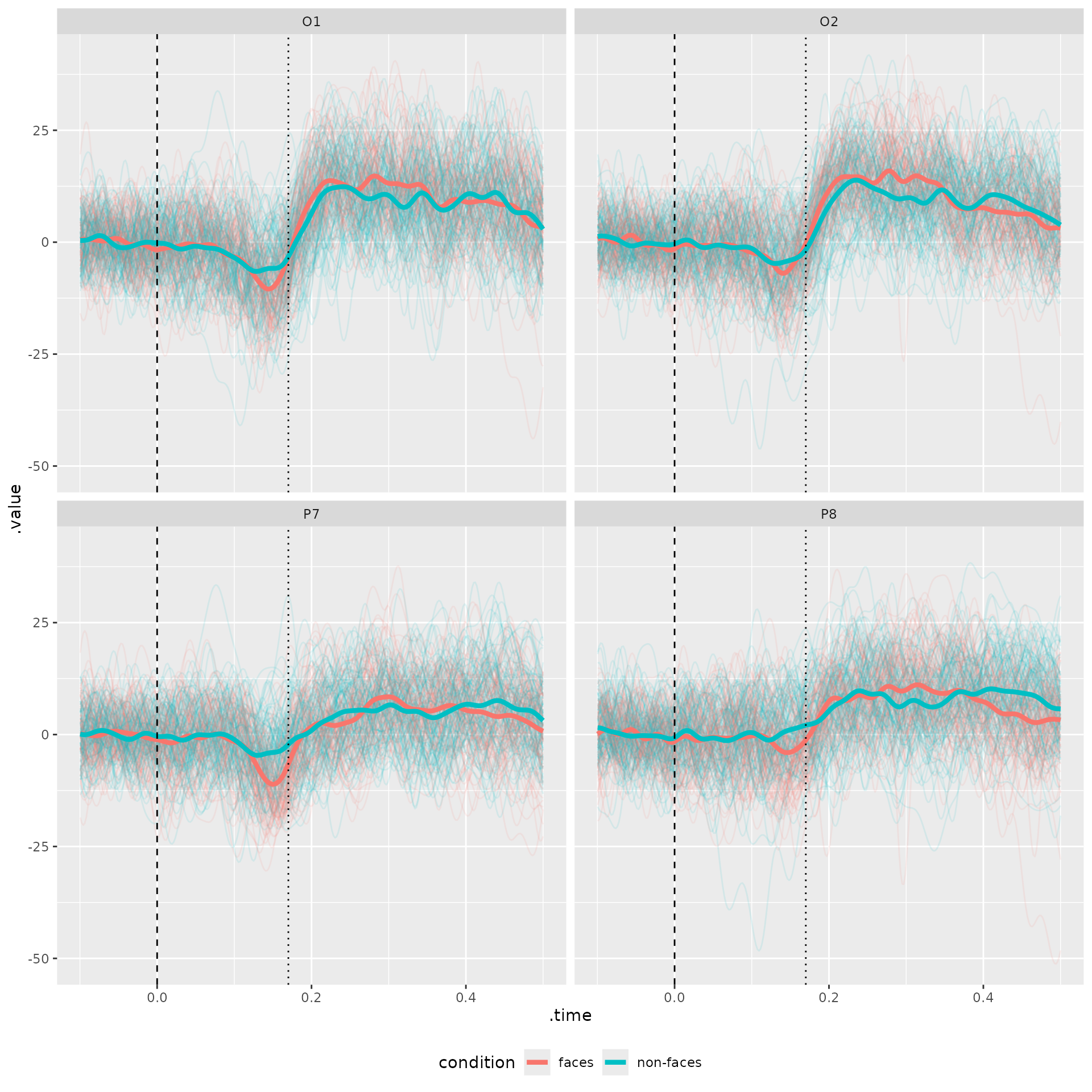
We can see here the N170 component in the faces condition for the
average trial on a single participant. We can investigate the signal by
averaging the channels of the occipital and parietal lobes using
transmute(), and the special function,
chs_mean(), a wrapper for rowMeans(), which
takes as arguments the relevant channels and whether missing values
should be omitted from the calculations.
faces_seg |>
  eeg_transmute(
    Occipital = chs_mean(across(starts_with("O")), na.rm = TRUE), #O1, O2, Oz
    Parietal = chs_mean(across(starts_with("O")), na.rm = TRUE) # P3, P4, P7, P8, Pz
  ) |>
  ggplot(aes(x = .time, y = .value)) +
  geom_line(alpha = .1, aes(group = .id, color = condition)) +
  stat_summary(
    fun = "mean", geom = "line", alpha = 1, size = 1,
    aes(color = condition)
  ) +
  facet_wrap(~.key) +
  theme(legend.position = "bottom")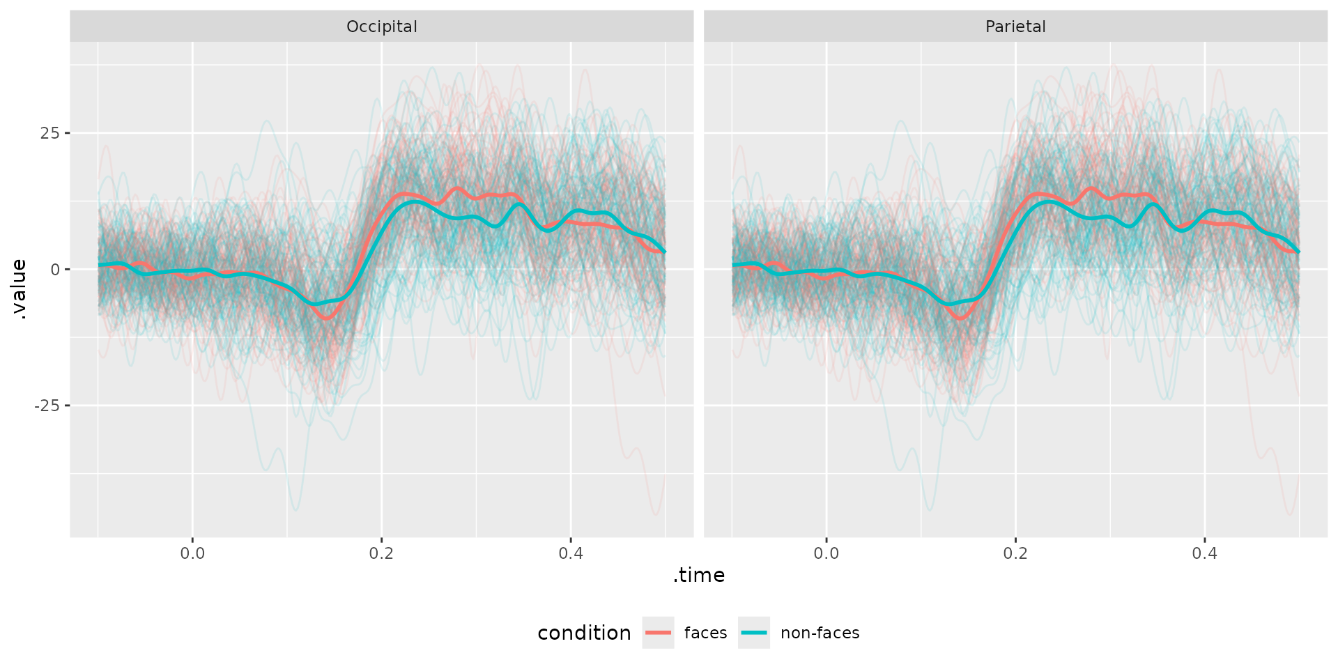
We can also calculate the ERPs and then plot them in their layout
(and we’ll add the same theme that plot uses for
eeg_lsts):
ERP_faces <- faces_seg |>
  eeg_group_by(.sample, condition) |>
  eeg_summarize(across_ch(mean, na.rm = TRUE))

ERP_plot <- ERP_faces |>
  ggplot(aes(x = .time, y = .value)) +
  geom_line(aes(color = condition)) +
  facet_wrap(~.key) +
  theme(legend.position = "bottom") +
  ggtitle("ERPs for faces vs non-faces") +
  theme_eeguana()

ERP_plot |> plot_in_layout()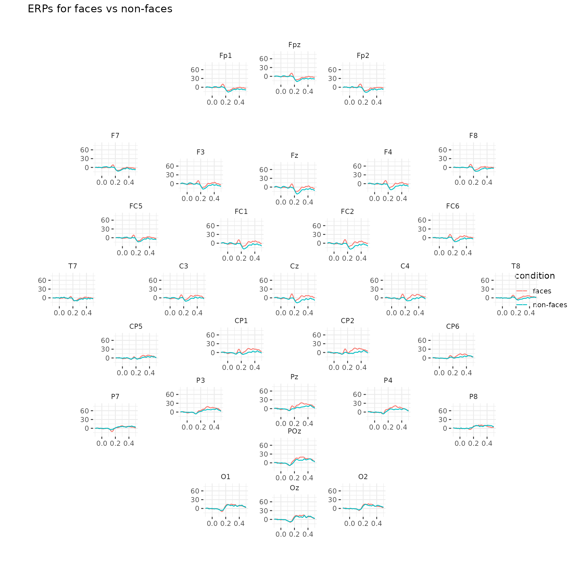
Another possibility is to create a topographic plot of the two
conditions, by first making segments that include only the interval
.1-.2 s after the onset of the stimuli, creating a table with
interpolated amplitudes and using the ggplot wrapper
plot_topo().
faces_seg |>
  eeg_filter(between(as_time(.sample, .unit = "s"), .1, .2)) |>
  eeg_group_by(condition) |>
  eeg_summarize(across_ch(mean, na.rm = TRUE)) |>
  plot_topo() +
  annotate_head() +
  geom_contour() +
  annotate_electrodes(colour = "black") +
  facet_grid(~condition)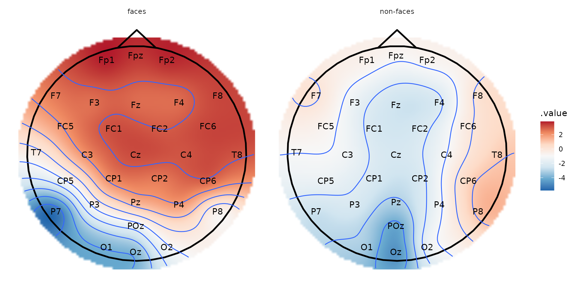
For more specialized plots or analyses, it might be necessary to extract the data in long data frame format first. Even though, we can do this without transforming the object, here, we transform the data first and then we visualize independent t-tests at every electrode and time point.
df <- faces_seg |>
  eeg_select(O1, O2, P7, P8) |>
  as_tidytable() |> #or alternatively as_tibble() if one uses dplyr
  # We can use regular dplyr/tidytable functions now
  group_by(.key, .time) |>
  summarize(
    `t-value` = t.test(
      .value[condition == "faces"],
      .value[condition == "non-faces"]
    )$statistic
  )

df
#> # A tidytable: 1,232 × 3
#> # Groups:      .key
#>    .key    .time `t-value`
#>    <chr>   <dbl>     <dbl>
#>  1 O1    -0.0996    0.204
#>  2 O1    -0.0977    0.227
#>  3 O1    -0.0957    0.234
#>  4 O1    -0.0938    0.219
#>  5 O1    -0.0918    0.173
#>  6 O1    -0.0898    0.0880
#>  7 O1    -0.0879   -0.0415
#>  8 O1    -0.0859   -0.221
#>  9 O1    -0.0840   -0.448
#> 10 O1    -0.0820   -0.713
#> # ℹ 1,222 more rows
Then we just load the data frame into ggplot.
ggplot(df, aes(x = .time, y = `t-value`)) + geom_line() +
  facet_wrap(~.key)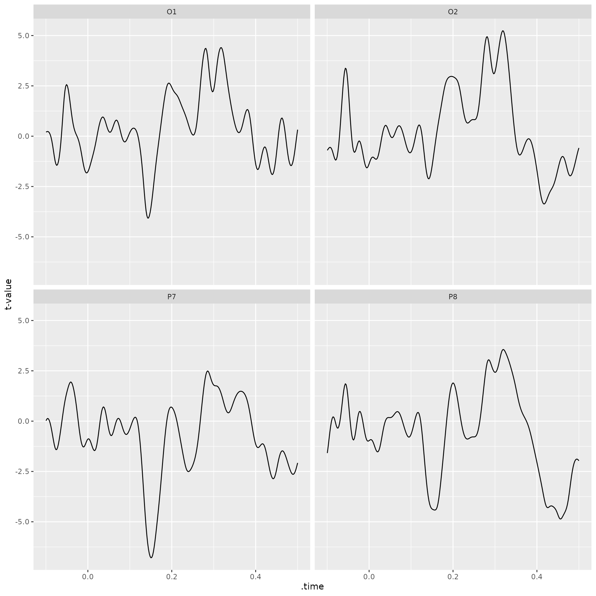
However, this can be also done in the without transforming the
eeg_lst object:
faces_seg_t <-
  faces_seg |>
  eeg_select(O1, O2, P7, P8) |>
  eeg_group_by(.sample) |>
  eeg_summarize(across_ch(list(t =  ~t.test(
    .[condition == "faces"],
    .[condition == "non-faces"]
  )$statistic)))

faces_seg_t |>
  ggplot(aes(x = .time, y = .value)) +
  geom_line(alpha = .1, aes(group = .id)) +
  stat_summary(fun = "mean", geom = "line", alpha = 1, size = 1) +
  facet_wrap(~.key) +
  theme(legend.position = "bottom")