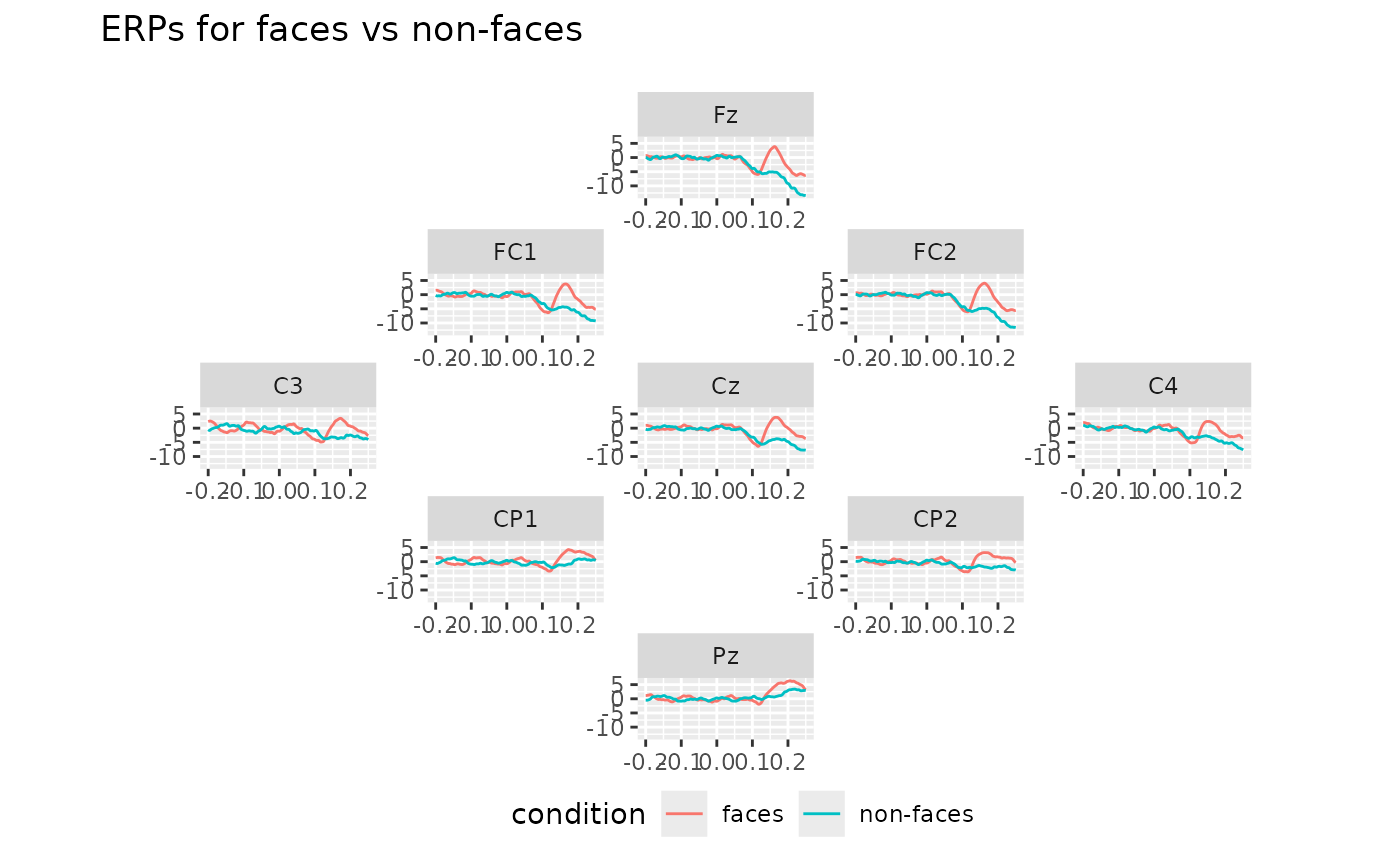
Arranges a ggplot so that the facet for each channel appears in its position on the scalp.
plot_in_layout(plot, ...)

# S3 method for gg
plot_in_layout(plot, .projection = "polar", .ratio = c(1, 1), ...)
Arguments
- plot
A ggplot object with channels
- ...
Not in use.
- .projection
.Projection type for converting the 3D coordinates of the electrodes into 2d coordinates. .Projection types available: "polar" (default), "orthographic", or "stereographic"
- .ratio
Ratio of the individual panels
Value
A ggplot object
Details
This function requires two steps: first, a ggplot object must be created with
ERPs faceted by channel (.key).
Then, the ggplot object is called in plot_in_layout. The function uses grobs
arranged according to .x .y coordinates extracted from the eeg_lst object, by
default in polar arrangement. The arrangement can be changed with the .projection
argument. White space in the plot can be reduced by changing ratio.
Additional components such as titles and annotations should be added to the
plot object using + exactly as you would for ggplot2::ggplot.
Title and legend adjustments will be treated as applying to the
whole plot object, while other theme adjustments will be treated as applying
to individual facets. x-axis and y-axis labels cannot be added at this stage.
See also
Other plotting functions:
annotate_electrodes(),
annotate_events(),
annotate_head(),
eeg_downsample(),
ggplot.eeg_lst(),
plot.eeg_lst(),
plot_components(),
plot_topo(),
theme_eeguana()
Other topographic plots and layouts:
layout_32_1020,
plot_components(),
plot_topo()
Examples
library(ggplot2)
# Create a ggplot object with some grand averaged ERPs
ERP_plot <- data_faces_ERPs %>%
  # select a few electrodes
  eeg_select(Fz, FC1, FC2, C3, Cz, C4, CP1, CP2, Pz) %>%
  # group by time point and condition
  eeg_group_by(.sample, condition) %>%
  # compute averages
  eeg_summarize(across_ch(mean, na.rm = TRUE)) %>%
  ggplot(aes(x = .time, y = .value)) +
  # plot the averaged waveforms
  geom_line(aes(color = condition)) +
  # facet by channel
  facet_wrap(~.key) +
  # add a legend and title
  theme(legend.position = "bottom") +
  ggtitle("ERPs for faces vs non-faces")

# Call the ggplot object with the layout function
plot_in_layout(ERP_plot)