Another example from a Fieldtrip tutorial: Preprocessing of EEG data and computing ERPs
Bruno Nicenboim
2024-03-12
Source:vignettes/preprocessing_erp.Rmd
preprocessing_erp.RmdThis tutorial is an adaptation (and some parts are a verbatim copy) of Fieldtrip’s Preprocessing - Reading continuous EEG data. Fieldtrip is a great MATLAB toolbox for MEG and EEG analysis. Here I show, how we would do a very similar analysis with eeguana. (No previous experience with Fieldtrip is needed to follow this vignette).
The preprocessing of data refers to the reading of the data, segmenting the data around interesting events such as triggers, temporal filtering, and optionally re-referencing.
There are largely two alternative approaches for preprocessing, which especially differ in the amount of memory required (and processing time). The first approach is to read all data from the file(s) into memory, apply filters, and subsequently cut the data into interesting segments. The second approach is to segment the data and then apply the filters to those segments only. This tutorial explains the second approach. It should be noticed that filtering distorts the edges of the segments, and this second approach should be followed with care.
Preprocessing involves several steps including identifying individual trials from the dataset, filtering and artifact rejections. This tutorial covers how to identify trials using the trigger signal. Defining data segments of interest can be done according to a specified trigger channel or according to your own criteria.
Dataset
The EEG dataset used in this script is available in Fieldtrip’s ftp. In the experiment, subjects made positive/negative or animal/human judgments on nouns. The nouns were either positive animals (puppy), negative animals (maggot), positive humans (princess), or negative humans (murderer). The nouns were presented visually (written words). The task cue (which judgment to make) was given with each word.
First we download the data:
download.file("https://download.fieldtriptoolbox.org/tutorial/preprocessing_erp/s04.eeg", "s04.eeg")
download.file("https://download.fieldtriptoolbox.org/tutorial/preprocessing_erp/s04.vhdr", "s04.vhdr")
download.file("https://download.fieldtriptoolbox.org/tutorial/preprocessing_erp/s04.vmrk", "s04.vmrk")
download.file("https://download.fieldtriptoolbox.org/tutorial/preprocessing_erp/mpi_customized_acticap64.mat", "mpi_customized_acticap64.mat")
And then we load the eeguana package and read the the
.vhdr fileinto memory. The function
read_vhdr() creates a list with data frames for the signal,
events, segments information, and incorporates in its attributes generic
EEG information.
data_judg <- read_vhdr(file = "s04.vhdr")
#> # Reading file s04.vhdr...
#> # Data from ./s04.eeg was read.
#> # Data from 1 segment(s) and 64 channels was loaded.
#> # Object size in memory 553.3 Mb
Procedure
Defining trials
The triggers were defined such that the trigger “S131” indicates
condition 1 (positive-negative judgment) and “S132” indicates condition
2 (animal-human judgment). We access the events with
events() function.
events_tbl(data_judg)
#>        .id       .type .description     .initial       .final .channel
#>      <int>      <char>       <char> <sample_int> <sample_int>   <char>
#>   1:     1 New Segment                         1            1     <NA>
#>   2:     1    Stimulus         S111        51507        51507     <NA>
#>   3:     1    Stimulus         S 11        51514        51514     <NA>
#>   4:     1    Stimulus         S123        52035        52035     <NA>
#>   5:     1    Stimulus         S141        52541        52541     <NA>
#>  ---
#> 957:     1    Stimulus         S112      1108150      1108150     <NA>
#> 958:     1    Stimulus         S106      1108157      1108157     <NA>
#> 959:     1    Stimulus         S122      1108169      1108169     <NA>
#> 960:     1    Stimulus         S141      1108929      1108929     <NA>
#> 961:     1    Stimulus         S132      1109582      1109582     <NA>
However, we want the ERP based on the trigger “S141” that precedes
any of these two triggers. We edit the events table (using dplyr
functions: mutate, case_when,
lead) to indicate to which condition each trigger “S141”
belongs, and then we can segment based on these conditions using
eeguana’s eeg_segment():
events_tbl(data_judg) <- mutate(events_tbl(data_judg),
  condition = case_when(
    .description == "S141" &
      lead(.description) == "S131" ~ 1,
    .description == "S141" &
      lead(.description) == "S132" ~ 2,
    TRUE ~ 0
  )
)
data_judg_s <- data_judg %>% eeg_segment(condition %in% c(1, 2), .lim = c(-0.2, 1))
#> # Total of 192 segments found.
#> # Object size in memory 57.4 Mb after segmentation.
Pre-processing and re-referencing
In this raw BrainVision dataset, the signal from all electrodes is
monopolar and referenced to the left mastoid. We want the signal to be
referenced to linked (left and right) mastoids. During the acquisition
the ‘RM’ electrode (number 32) had been placed on the right mastoid. We
first baseline the signal with eeg_baseline(). In order to
re-reference the data (e.g. including also the right mastoid in the
reference) we add implicit channel ‘REF’ to the channels (which
represents the left mastoid) by creating a channel with
channel_dbl() and filling it with zeros using
eeg_mutate() overloaded by eeguana to work with
eeg_lst's (see ?`dplyr-eeguana`). The we
re-reference the data using ‘REF’ and ‘RM’, the left and right mastoids
respectively using eeg_rereference(). Finally we apply a
low-pass filter with a stop band frequency of 100 Hz using
eeg_filt_low_pass():
data_judg_s <- data_judg_s %>%
# From the beginning of our desired segment length:
eeg_baseline(.lim = -.2) %>%
# The reference channel REF is filled with 0
eeg_mutate(REF = channel_dbl(0)) %>%
# All channels are references with REF
eeg_rereference(.ref = c("RM", "REF"))
data_judg_s_p <- data_judg_s %>%
# A low pass filter is applied
eeg_filt_low_pass(.freq = 100)
#> Setting up low-pass filter at 100 Hz
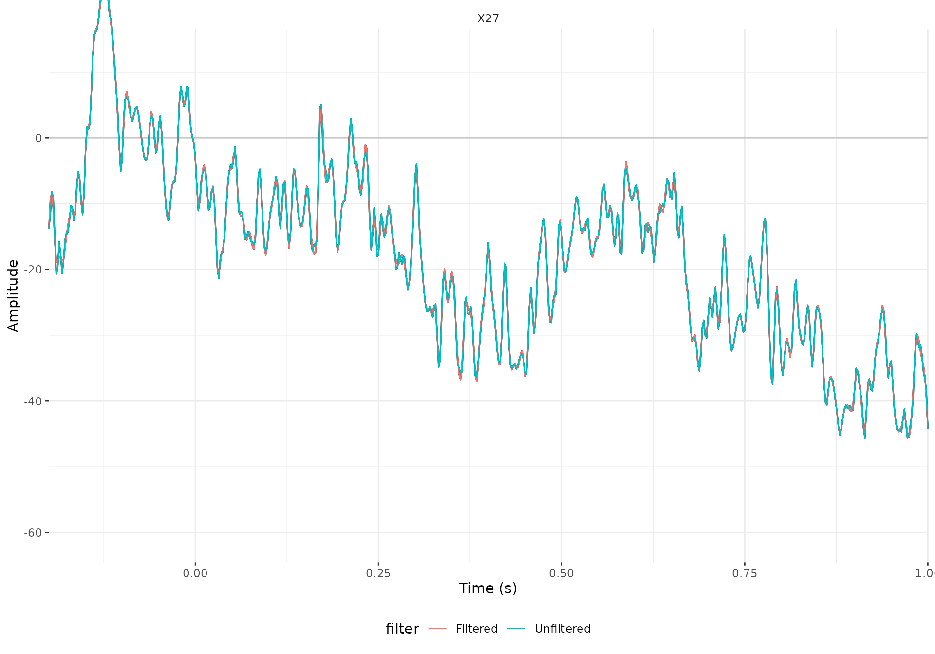
#> Width of the transition band at the high cut-off frequency is 25 HzWe can have a look at one of the trials (the second one) of one
channel (channel 27). We eeg_filter() the desired segment
(meaning to select rows or samples, do not confuse with filtering the
signal, e.g., eeg_filt_low_pass()) and
eeg_select() the channel, then we add information
indicating if we are looking at the filtered or unfiltered data. Finally
we bind both eeg_lst's and we use use plot()
to generate a default ggplot:
X27_filtered <- data_judg_s_p %>%
  eeg_filter(segment == 2) %>%
  eeg_select(X27) %>%
  eeg_mutate(filter = "Filtered")

X27_unfiltered <- data_judg_s %>%
  eeg_filter(segment == 2) %>%
  eeg_select(X27) %>%
  eeg_mutate(filter = "Unfiltered")

eeg_bind(X27_filtered, X27_unfiltered) %>%
  plot() +
  geom_line(aes(color = filter)) +
  facet_wrap(~.key) +
  theme(legend.position = "bottom")
#> # Object size in memory 30.4 Kb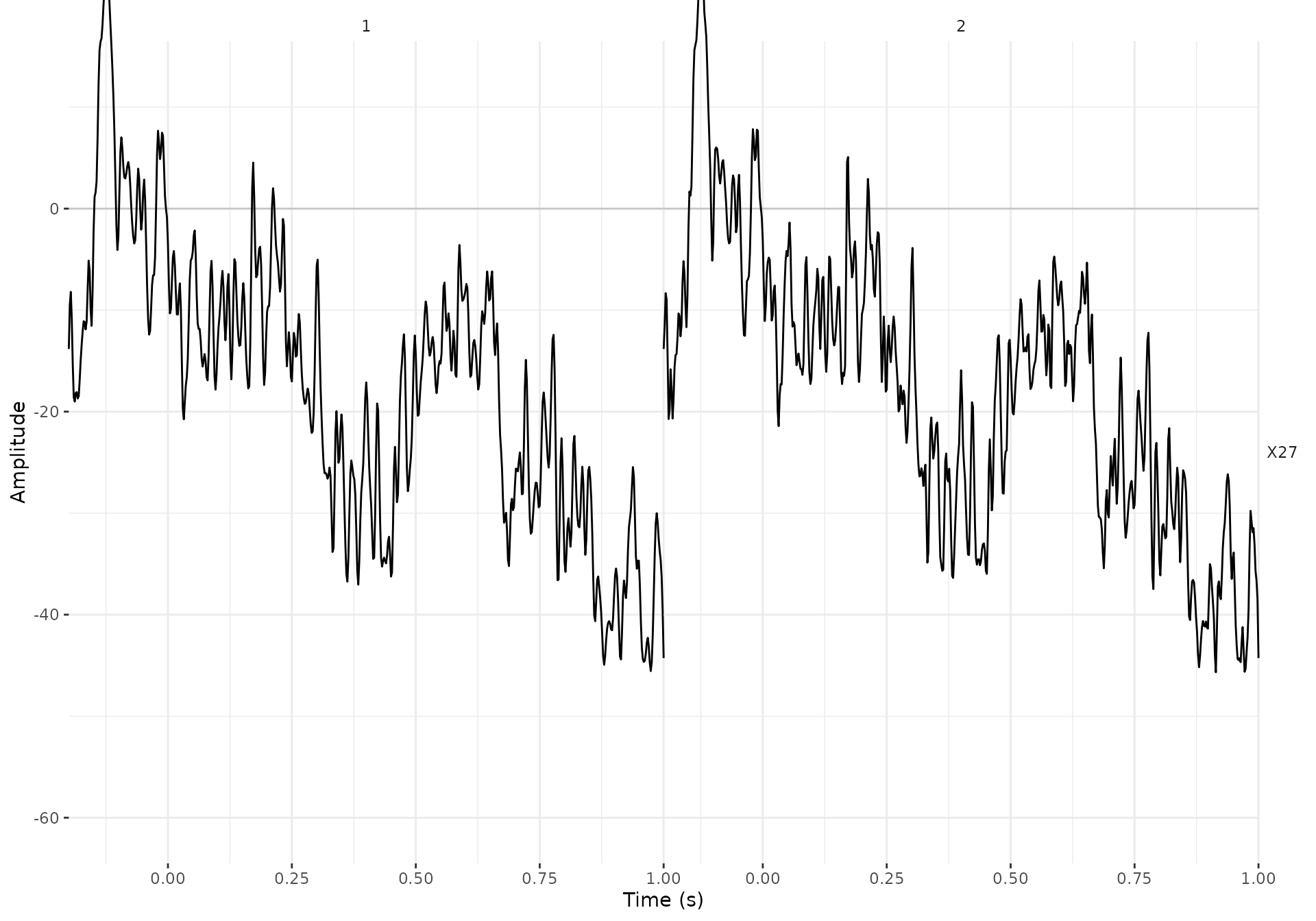
Extracting the EOG signals
In the BrainAmp acquisition system, all channels are measured relative to a common reference. For the horizontal EOG we will compute the potential difference between channels 57 and 25 (see the plot of the layout and the figure below). For the vertical EOG we will use channel 53 and channel “LEOG” which was placed below the subjects’ left eye.
data_judg_s_p <- data_judg_s_p %>%
  eeg_rereference(LEOG, .ref = "X53") %>%
  eeg_rereference(X25, .ref = "X57") %>%
  eeg_rename(eogv = LEOG, eogh = X25) %>%
  eeg_select(-X53, X57)
You can check the channel labels that are now present in the data:
channel_names(data_judg_s_p)
#>  [1] "X1"   "X2"   "X3"   "X4"   "X5"   "X6"   "X7"   "X8"   "X9"   "X10"
#> [11] "X11"  "X12"  "X13"  "X14"  "X15"  "X16"  "X17"  "X18"  "X19"  "X20"
#> [21] "X21"  "X22"  "X23"  "X24"  "eogh" "X26"  "X27"  "X28"  "X29"  "X30"
#> [31] "X31"  "RM"   "X33"  "X34"  "X35"  "X36"  "X37"  "X38"  "X39"  "X40"
#> [41] "X41"  "X42"  "X43"  "X44"  "X45"  "X46"  "X47"  "X48"  "X49"  "X50"
#> [51] "X51"  "X52"  "X54"  "X55"  "X56"  "X57"  "X58"  "X59"  "X60"  "eogv"
#> [61] "X62"  "X63"  "X64"  "REF"
Artifacts
A next important step of EEG preprocessing is detection (and
rejection) of artifacts. We can plot EOG channel (‘veog’, number 61) and
confirm that the segments 22, 42, 126, 136 and 150 contain blinks. We
use here ggplot(), which is more flexible than
plot().
data_judg_s_p %>%
  eeg_select(eogv) %>%
  ggplot(aes(x = .time, y = .value)) +
  geom_line() +
  facet_wrap(~segment) +
  theme(axis.text.x = element_text(angle = 90)) +
  scale_x_continuous(breaks = seq(0, 1, .2)) +
  theme_eeguana()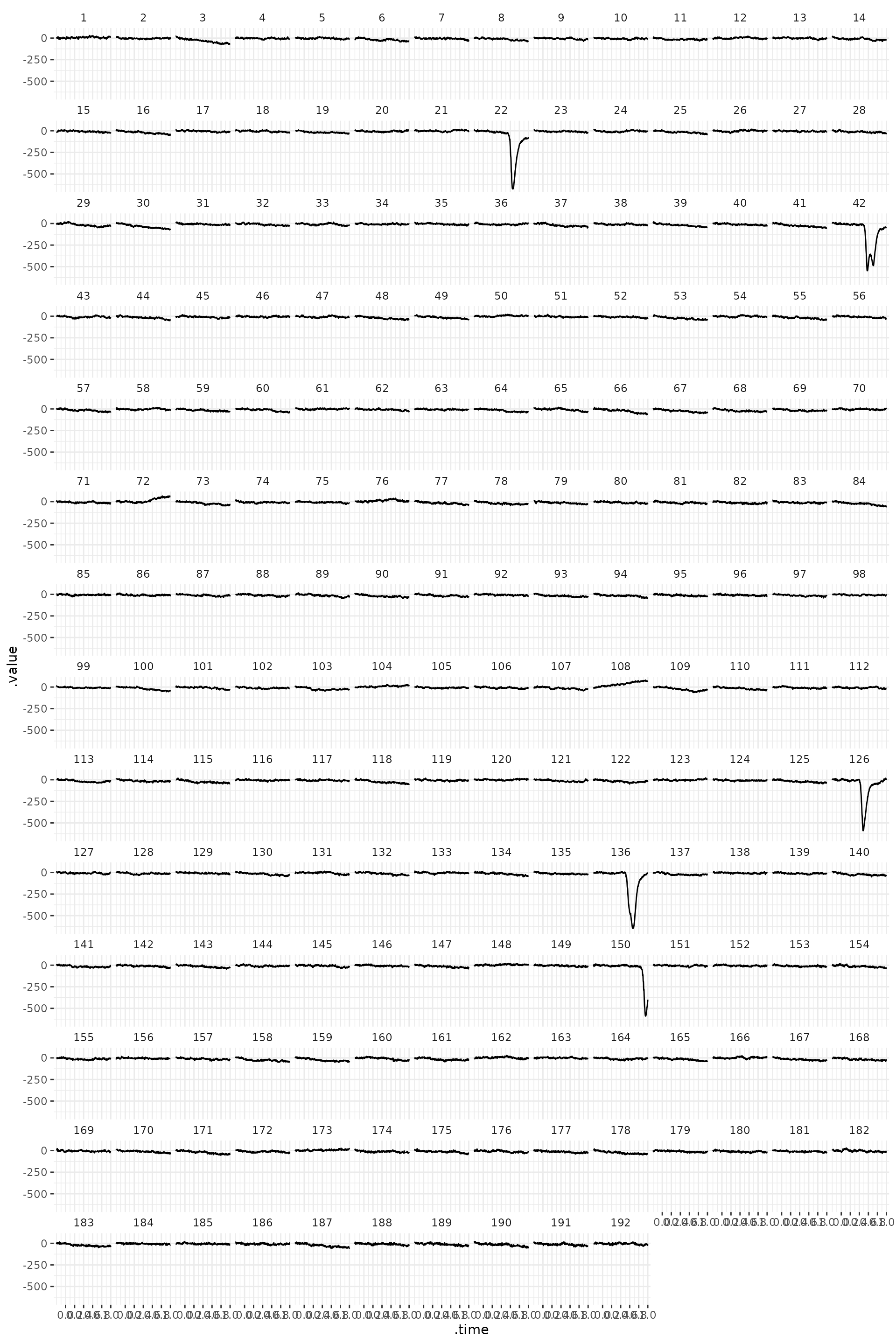
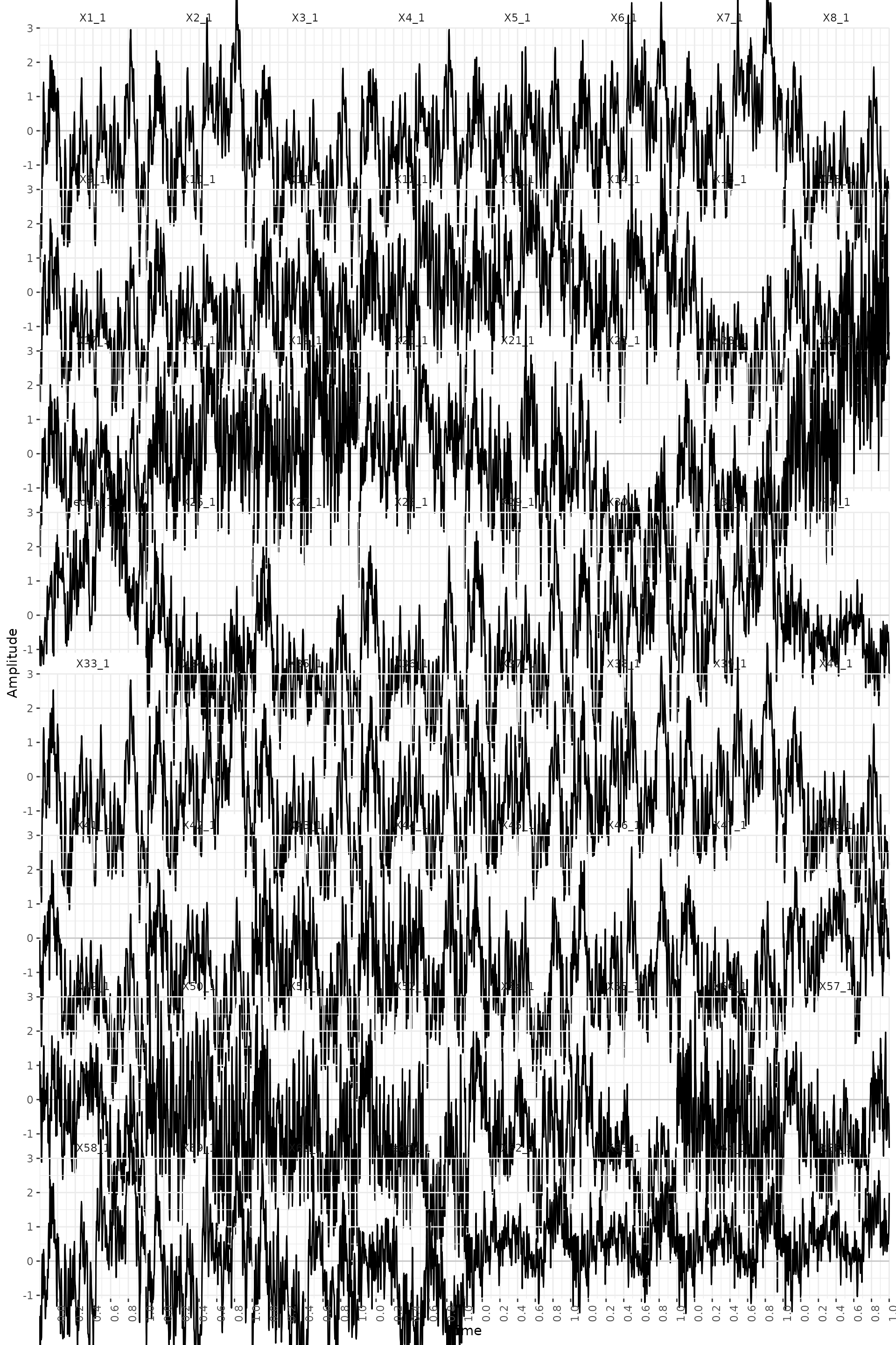
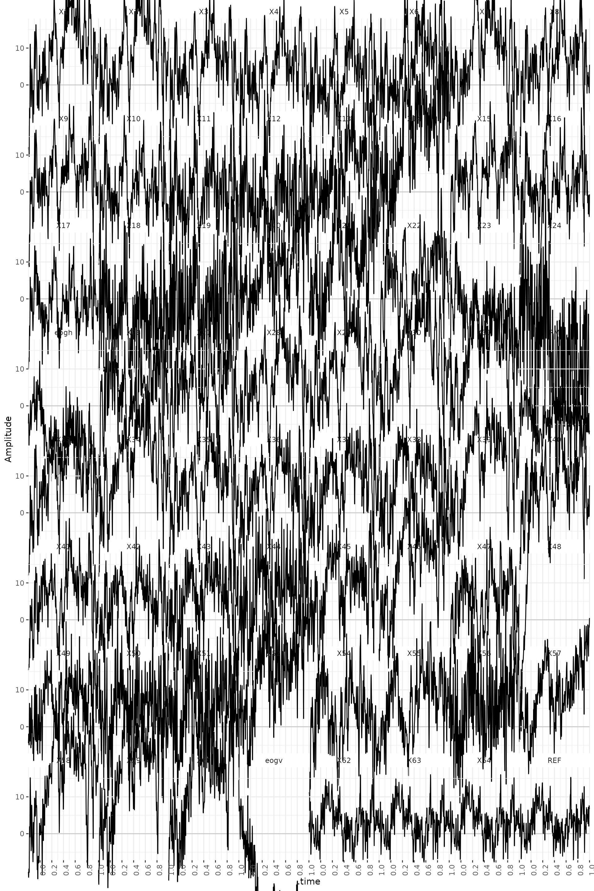
The data can be also displayed in a different way. And
ggplotly() can help us navigate the data. One quirk we need
to take into account is that mean operations such as, min,
max, var (but not mean) remove
the properties of the channels. Rather than use this functions directly
we use them in the following way ~ channel_dbl(fn(.)),
where fn is a placeholder:
data_summary <- data_judg_s_p %>%
  eeg_select(-eogh, -eogv) %>%
  eeg_group_by(segment) %>%
  eeg_summarize(across_ch(~ channel_dbl(var(.))))

plot_general <- data_summary %>%
  ggplot(aes(x = segment, y = .key, fill = .value)) +
  geom_raster() +
  theme(legend.position = "none", axis.text.y = element_text(size = 6))

plot_channels <- data_summary %>%
  eeg_ungroup() %>%
  eeg_summarize(across_ch(~ channel_dbl(max(.)) )) %>%
  ggplot(aes(x = .value, y = .key)) +
  geom_point() +
  theme(axis.text.y = element_text(size = 6))

plot_segments <- data_summary %>%
  chs_fun(max) %>%
  ggplot(aes(x = segment, y = .value)) +
  geom_point() +
  theme(axis.text.y = element_text(size = 6))

subplot(ggplotly(plot_general), ggplotly(plot_channels), ggplotly(plot_segments), nrows = 2)
Here, we have plotted the trial 90 -the one with the highest variance. We can see a drift in the channel 48.
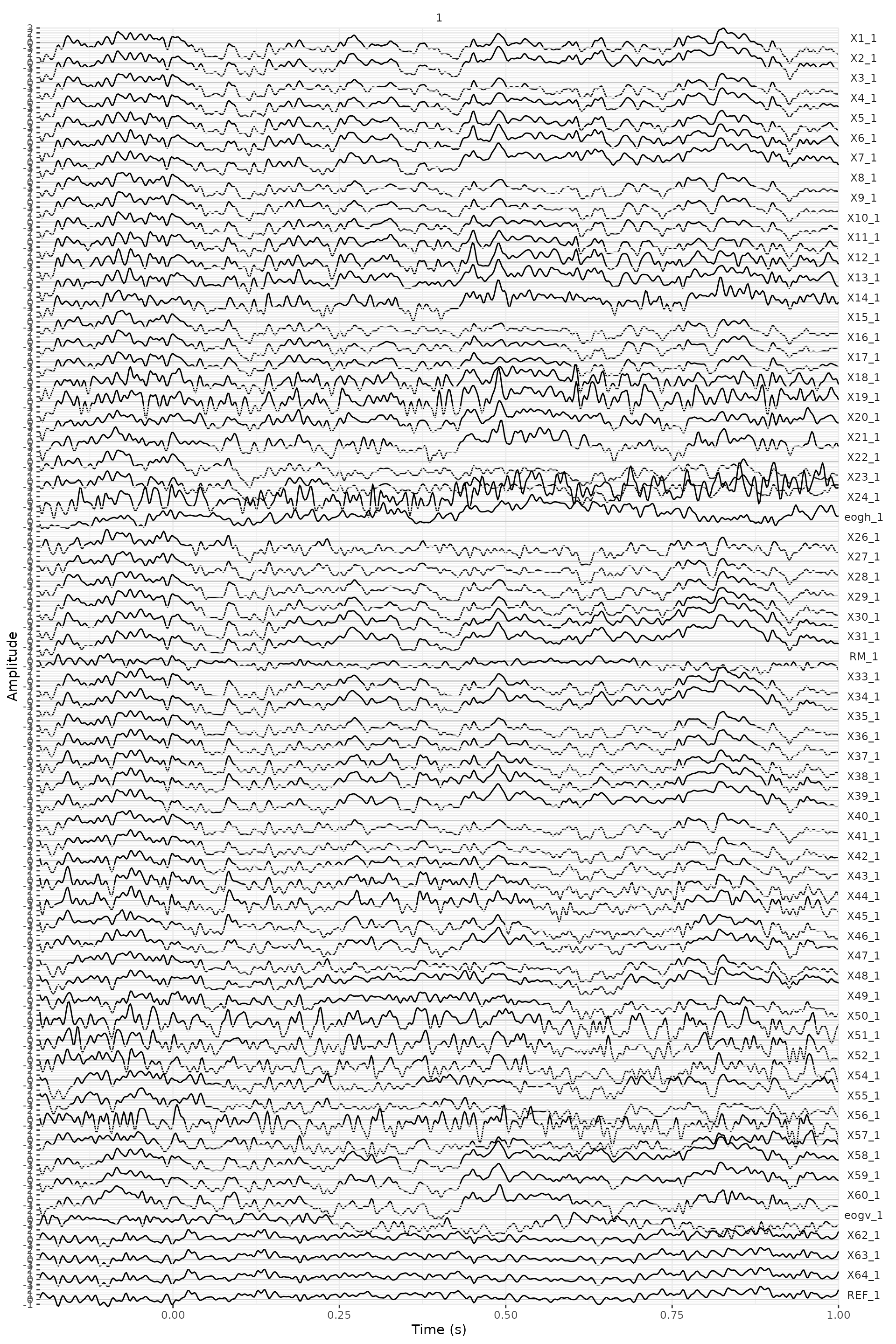
data_judg_s_p %>%
  eeg_filter(segment == 90) %>%
  plot() +
  facet_wrap(~.key) +
  theme(axis.text.x = element_text(angle = 90)) +
  scale_x_continuous(breaks = seq(0, 1, .2))
#> Scale for x is already present.
#> Adding another scale for x, which will replace the existing scale.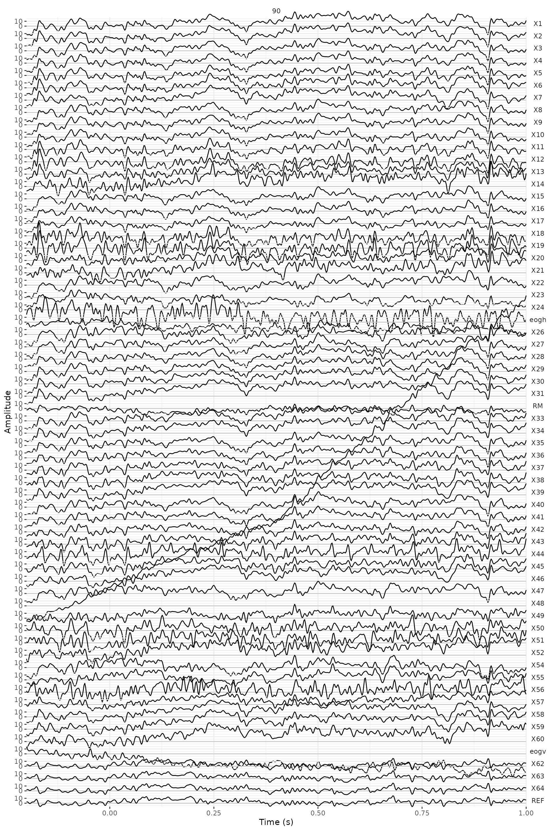
Rejection of trials based on visual inspection is somewhat arbitrary. Sometimes it is not easy to decide if a trial has to be rejected or not. In this exercise we suggest that you remove 8 trials with the highest variance (trial numbers 22, 42, 89, 90, 92, 126, 136 and 150): the trials with blinks that we saw before.
data_judg_s_p <- data_judg_s_p %>%
  eeg_filter(!segment %in% c(22, 42, 89, 90, 92, 126, 136, 150))
Computing and plotting the ERP’s
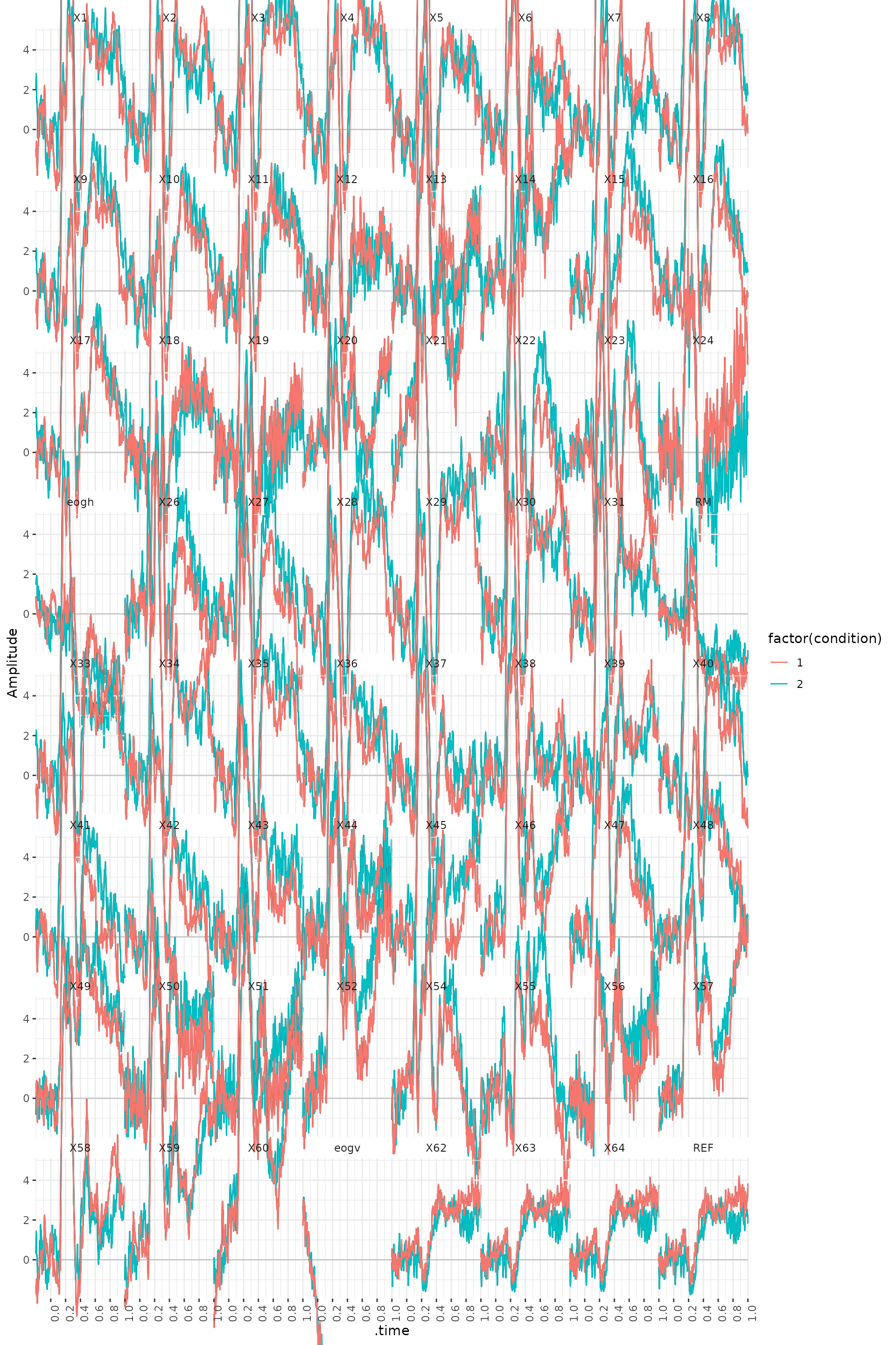
We now would like to compute the ERP’s for two conditions:
positive-negative judgment and human-animal judgment. This is
straightforward to do with eeg_group_by() and
eeg_summarize() with across_ch().
ERPs <- data_judg_s_p %>%
  eeg_group_by(.sample, condition) %>%
  eeg_summarize(across_ch(mean, na.rm = TRUE))

ERPs %>%
  plot() +
  geom_line(aes(color = factor(condition))) +
  facet_wrap(~.key) +
  theme(axis.text.x = element_text(angle = 90)) +
  scale_x_continuous(breaks = seq(0, 1, .2))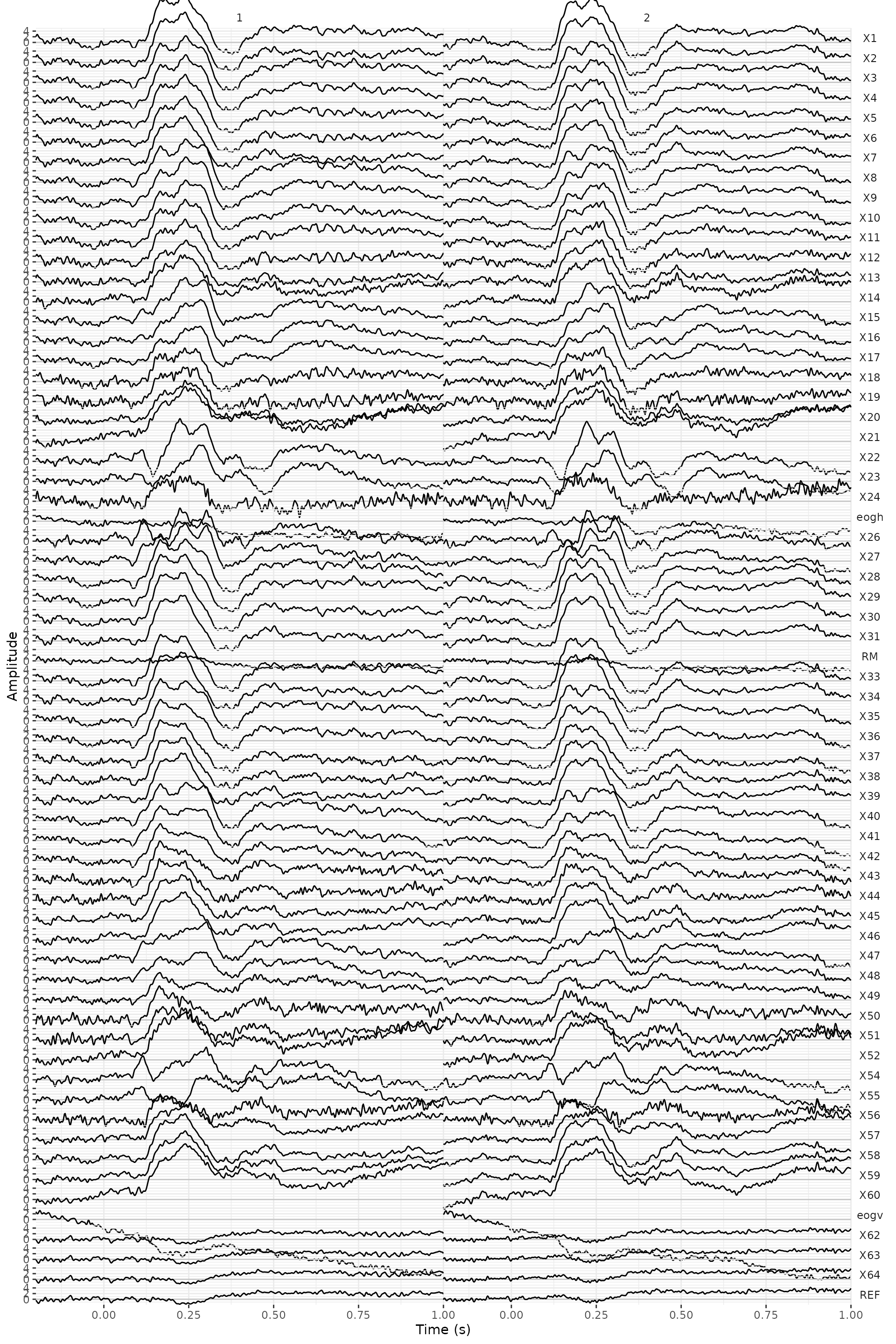
The following code allows you to look at the ERP difference waves.
diff_ERPs <- data_judg_s_p %>%
  eeg_group_by(.sample) %>%
  eeg_summarize(across_ch(list(~
  mean(.[condition == 1] - .[condition == 2],
    na.rm = TRUE
  ))))

diff_ERPs %>%
  plot() +
  geom_line() +
  facet_wrap(~.key) +
  theme(axis.text.x = element_text(angle = 90)) +
  scale_x_continuous(breaks = seq(0, 1, .2))