Categories: stats / Tags: stan Bayesian r /
Update Feb 1st, 2024: I updated the Stan syntax.
⚠️ This post is NOT about “Masheen Lurning”: I’m spelling it like this to avoid luring visitors into this post for the wrong reasons. In the context of “Masheen Lurning”, one teaches a “masheen” to make the most rewarding decisions. In contrast, this post is about fitting human (or possibly also animal) data with decisions made along a number of trials assuming that some type of reinforcement learning occurred.⚠️
I’ll focus on a Bayesian implementation of Q-learning using Stan. Q-learning is a specific type of reinforcement learning (RL) model that can explain how humans (and other organisms) learn behavioral policies (to make decisions) from rewards. Niv (2009) presents a very extensive review of RL in the brain. Readers interested in The Book about RL should see Sutton and Barto (2018).
I will mostly follow the implementation of van Geen and Gerraty (2021), who present a tutorial on a hierarchical Bayesian implementation of Q-learning. However, I think there are places where a different parametrization would be more appropriate. I will also model my own simulated data, especially because I wanted to check if I’m doing things right. Another useful tutorial about Bayesian modeling of RL is Zhang et al. (2020), however, that tutorial uses a Rescorla–Wagner model, rather than Q-learning. Before you continue reading, notice that if you just want to fit data using a RL model and don’t care about the nitty gritty details, you can just use the R package hBayesDM.
The rest of the post is about simulating one subject doing an experiment and fitting it with Stan, and then simulating several subjects doing the same experiment and fitting that data with Stan.
First, I’m going to load some R packages that will be useful throughout this post and set a seed, so that the simulated data will be always the same.
library(dplyr) # Data manipulation
library(tidyr) # To pivot the data
library(purrr) # List manipulation
library(ggplot2) # Nice plots
library(extraDistr) # More distributions
library(MASS) # Tu use the multinormal distribution
library(cmdstanr) # Lightweight Stan interface
library(bayesplot) # Nice Bayesian plots
set.seed(123)
Restless bandits or slot machines with non-fixed probabilities of a reward
I simulate data from a two-armed restless bandit, where the arms are independent. This is basically as if there were two slot machines that offer rewards with probabilities that vary with time following a random walk. I always wondered why so many researchers are modeling slot machines, but it turns out they can actually represent realistic options in life. There is a post from Speekenbrink lab that gives context to the restless bandits (and they also simulate data from a different RL algorithm).

I set up here a restless bandit with 2 arms that runs over 1000 trials. The reward, \(R_{t,a}\), for the time step or trial \(t\) for the arm \(a\) follows a random walk and it’s defined as follows:
For \(t =1\), \[\begin{equation} R_{t,a} \sim \mathit{Normal}(0, \sigma) \end{equation}\]
For \(t >1\),
\[\begin{equation} R_{t,a} \sim \mathit{Normal}(R_{t-1,a}, \sigma) \end{equation}\]
with \(\sigma = .1\)
In R, this looks as follows.
# set up
N_arms <- 2
N_trials <- 1000
sigma <- .1
## Reward matrix:
# First define a matrix with values sampled from Normal(0, sigma)
R <- matrix(rnorm(N_trials * N_arms, mean = 0, sd = sigma),
            ncol = N_arms)
# Then I do a cumulative sum over the rows (MARGIN = 2)
R <- apply(R, MARGIN = 2, FUN = cumsum)
colnames(R) <- paste0("arm_", 1:N_arms)
The first rows of the reward matrix will look like this:
head(R) arm_1 arm_2
[1,] -0.056 -0.10
[2,] -0.079 -0.20
[3,] 0.077 -0.21
[4,] 0.084 -0.22
[5,] 0.097 -0.47
[6,] 0.268 -0.37In this simulated experiment, a subject is presented at each trial with two choices, to either select arm one or arm two. Each time they’ll get a reward (or a negative reward, that is, a punisment) determined by a random walk simulated before in the matrix \(R\).
Some tidyr to plot the rewards.
d_exp <- R %>%
  as_tibble() %>%
  pivot_longer(cols = everything(),
               names_to = "arm",
               values_to = "reward") %>%
  group_by(arm) %>%
  mutate(trial = 1:n())
ggplot(d_exp, aes(x = trial, y = reward, color = arm)) +
  geom_line()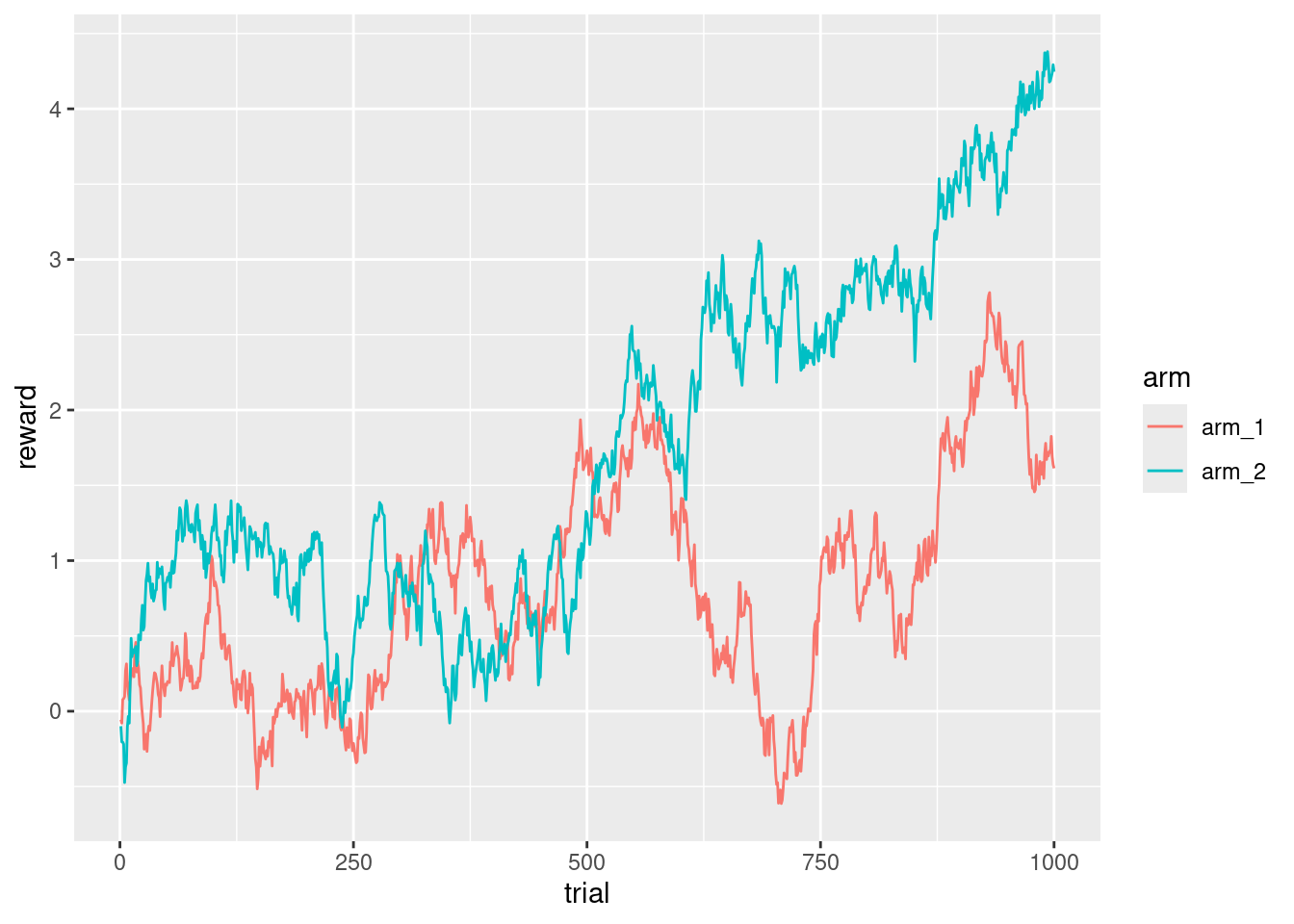
I see that the arm that will give better rewards depends on the trial, and that a subject should keep exploring at least until trial ~650 to verify that they are not exploiting the wrong arm. There are many, many variations of the bandits, some of them give a fixed reward with some probability based on the random walk, sometimes there are more arms, and all of them are presented as choices, and in some other tasks only a random subset of the arms are presented to the subject.
Simulating actions using Q-learning
There are also many, many RL models. Q-learning is a type of RL model where an agent (e.g., a human subject) learns the predictive value (in terms of future expected rewards) of taking a specific action (e.g., choosing arm one or two of the bandit) at a certain state (here, at a given trial), \(t\). This predictive value is denoted as \(Q\). In a simplified model of Q-learning, the actions of a subject will depend (to some extent) on \(Q\).
Let’s focus on the case of two arms:
- For \(t = 1\)
In the first trial, \(Q\) will be initialized with the same value for each action (e.g., \(0.5\)), and the subject will take an action with probability \(\theta\) based on their bias to one of the arms. I use \(\beta_{0}\) as the bias to arm 2. This parameter can vary freely, \([-\infty,\infty]\), and it’s converted to the \([0,1]\) range using \(logit^{-1}\). If there are more arms presented one should use a \(softmax\) function instead.
\[\begin{equation} \begin{aligned} Q_{t=1,a = 1} &= .5 \\ Q_{t=1,a = 2} &= .5 \\ \theta &= logit^{-1}(\beta_0) \end{aligned} \end{equation}\]
Whether the subject decides arm 1 or arm 2 depends on \(\theta\):
\[\begin{equation} action \sim \begin{cases} 1 \text{ with probability } 1-\theta_t\\ 2 \text{ with probability } \theta_t \end{cases} \end{equation}\]
Now I update the \(Q\) value that corresponds to the action taken for the next trial. Here, \(\alpha\), the learning rate, determines the extent to which the prediction error will play a role in updating an action’s value. This prediction error is quantified as the difference between the expected value of an action and the actual reward on a given trial, \((R_t - Q_{t, a})\). The parameter \(\alpha\) is bounded between \([0,1]\) to identify the model.1 Higher values of \(\alpha\) imply greater sensitivity to the most recent choice outcome, that is the most recent reward.
\[\begin{equation} Q_{t + 1,action} = Q_{t, action} + \alpha \cdot (R_{t,action} - Q_{t, action}) \end{equation}\]
For the action non taken, \(-action\), the value of \(Q\) remains the same (in the first trial, that would be 0.5):
\[\begin{equation} Q_{t + 1, -action} = Q_{t, -action} \end{equation}\]
- For \(t >1\) things get more interesting: the influence of \(Q\) in the agent behavior is governed by an inverse temperature parameter (\(\beta_1\)). Smaller values of \(\beta_1\) lead to a more exploratory behavior.
The idea will be that we obtain the probability, \(\theta\), of a specific action in a given trial based on two factors: that action’s value, \(Q\) in that trial (learned through its reward history), and how influential this value will be in determining the action taken. Again, because there are only two choices we can use \(logit^-1\) function, if we had more choices we would use a \(softmax\) function.
\[\begin{equation} \theta_t = logit^{-1}(\beta_0 + \beta_1 \cdot (Q_{t,2} - Q_{t,1})) \end{equation}\]
Again, and for every trial, whether the subject decides arm 1 or arm 2 depends on \(\theta\): \[\begin{equation} action \sim \begin{cases} 1 \text{ with probability } 1-\theta_t\\ 2 \text{ with probability } \theta_t \end{cases} \end{equation}\]
And \(Q\) gets updated for the next trial:
\[\begin{equation} \begin{aligned} Q_{t + 1,a = action} &= Q_{t, action} + \alpha \cdot (R_{t,action} - Q_{t, action})\\ Q_{t + 1,a = -action} &= Q_{t, -action} \end{aligned} \end{equation}\]
The following R code implements these equations:
# True values
alpha <- .3 # learning rate
beta_0 <- 0.5 # bias to arm "b"
beta_1 <- 3 # inverse temperature
# Q vector with the first value set at 0.5
# True Q matrix, it has an extra row,
# since it keeps updating also for trial N_trial + 1
Q <- matrix(nrow = N_trials + 1, ncol = N_arms)
Q[1, ] <- rep(.5, N_arms) # initial values for all Q
action <- rep(NA, times = N_trials)
theta <- rep(NA, times = N_trials)
for (t in 1:N_trials) {
  # probability of choosing arm_2
  theta[t] <- plogis(beta_0 + beta_1 * (Q[t, 2] - Q[t, 1]))
  # What the synthethic subject would respond,
  # with 1 indicating arm 1, and 2 indicating arm 2
  action[t] <- rbern(1, theta[t]) + 1
  Q[t + 1, action[t]] <- Q[t, action[t]] +
    alpha * (R[t, action[t]] - Q[t, action[t]])
  nonactions_t <- (1:N_arms)[-action[t]]
  Q[t + 1, nonactions_t] <- Q[t, nonactions_t]
}
This is what I’m generating trial by trial:
tibble(Q[1:N_trials, ], R, action)# A tibble: 1,000 × 3
`Q[1:N_trials, ]`[,1] [,2] R[,"arm_1"] [,"arm_2"] action
<dbl> <dbl> <dbl> <dbl> <dbl>
1 0.5 0.5 -0.0560 -0.0996 2
2 0.5 0.320 -0.0791 -0.204 1
3 0.326 0.320 0.0768 -0.205 2
4 0.326 0.162 0.0839 -0.219 1
5 0.254 0.162 0.0968 -0.474 2
6 0.254 -0.0283 0.268 -0.369 2
7 0.254 -0.131 0.314 -0.344 1
8 0.272 -0.131 0.188 -0.103 2
9 0.272 -0.122 0.119 -0.0344 1
10 0.226 -0.122 0.0746 -0.0791 1
# ℹ 990 more rowsLet’s see what would this subject choose in each trial.
d_res <- tibble(
  arm = ifelse(action == 1, "arm_1", "arm_2"),
  trial = 1:N_trials
) %>%
  left_join(d_exp)
ggplot(d_exp, aes(x = trial, y = reward, color = arm)) +
  geom_line() +
  geom_point(
    data = d_res,
    aes(x = trial, y = reward),
    color = "black",
    shape = 1
  )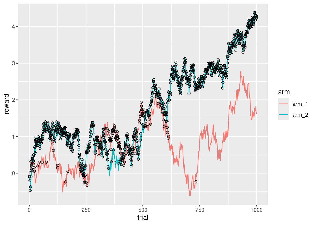
It’s interesting that there is a point (around the trial 650), where the second arm is so clearly better than the first arm, that it makes almost no sense to keep exploring.
What will be the reward of this subject?
sum(d_res$reward)[1] 1788What will be the maximum possible reward?
sum(apply(R, MARGIN = 1, FUN = max))[1] 1846Now let’s fit the model in Stan. A major difference with the R code is that I don’t keep track of all the Q values. I just keep track of one Q value for each arm, and I update them at the end of every trial. Also I store the difference between them in the vector Q_diff.
  vector[N_arms] Q = [.5, .5]';
  vector[N_trials] Q_diff;
  for(t in 1:N_trials){
    Q_diff[t] = Q[2] - Q[1];
    Q[action[t]] += alpha * (R[t, action[t]] - Q[action[t]]);
  }
The complete code is shown below.
data {
  int<lower=0> N_trials;
  array[N_trials] int action;
  int N_arms;
  matrix[N_trials,N_arms] R;
}
transformed data {
  array[N_trials] int response;
  for(n in 1:N_trials)
    response[n] = action[n] - 1;
}
parameters {
  real<lower = 0, upper = 1> alpha;
  real beta_0;
  real beta_1;
}
model {
  vector[N_arms] Q = [.5, .5]';
  vector[N_trials] Q_diff;
  for(t in 1:N_trials){
    Q_diff[t] = Q[2] - Q[1];
    Q[action[t]] += alpha * (R[t, action[t]] - Q[action[t]]);
  }
  target += beta_lpdf(alpha | 1, 1);
  target += normal_lpdf(beta_0 | 2, 5);
  target += normal_lpdf(beta_1 | 0, 1);
  target += bernoulli_logit_lpmf(response | beta_0 + beta_1 * Q_diff);
}
I compile the model and fit it.
m_ql <- cmdstan_model("qlearning.stan")
fit_ql <- m_ql$sample(
  data = list(
    action = action,
    N_trials = N_trials,
    N_arms = N_arms,
    R = R
  ),
  parallel_chains = 4
)
The sampling is super fast, just a couple of seconds. In this case, compiling the model was slower than sampling.
fit_ql$summary(c("alpha", "beta_0", "beta_1"))# A tibble: 3 × 10
variable mean median sd mad q5 q95 rhat ess_bulk ess_tail
<chr> <dbl> <dbl> <dbl> <dbl> <dbl> <dbl> <dbl> <dbl> <dbl>
1 alpha 0.266 0.261 0.0497 0.0469 0.196 0.355 1.00 2258. 1790.
2 beta_0 0.586 0.586 0.119 0.121 0.390 0.782 1.00 2906. 3191.
3 beta_1 2.98 2.97 0.246 0.243 2.59 3.39 1.00 2704. 2881.The recovery of the parameters seems fine.
mcmc_recover_hist(fit_ql$draws(c("alpha", "beta_0", "beta_1")),
  true = c(alpha, beta_0, beta_1)
)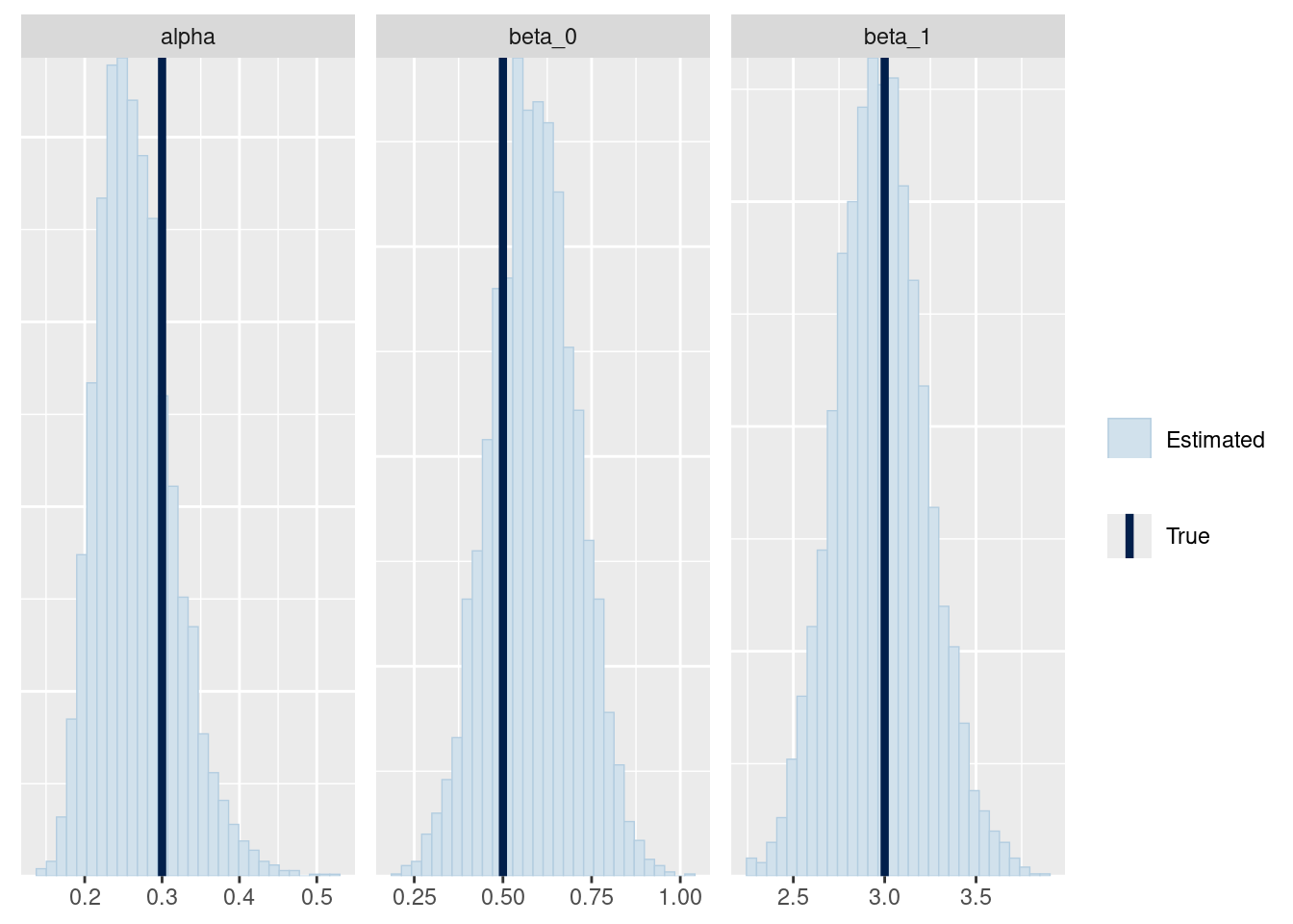
Either my Stan model was correct or I made the same mistakes in the R code and in the Stan model.2
A hierarchical Q-learning model
Now let’s try to implement this hierarchically. I have several subjects (N_subj), they all have their own bias, their own learning rate, and their own inverse temperature, but these values are not that different from subject to subject (there is shrinkage). I also assume that somehow these three parameters are mildly correlated, people with more bias also have a stronger learning rate and inverse temperature.
Here, I diverge a bit from the model of van Geen and Gerraty (2021). I just assume that all the individual differences are generated from the same multinormal distribution. This allows me to model the variance (or SD) of the parameters and to assume that they could be correlated (or not).
This means that in the hierarchical model, rather than \(\alpha\) I use \(\alpha + u_{i,1}\), rather than \(\beta_0\), \(\beta_0 + u_{i,2}\), and rather than \(\beta_1\), \(beta_1 + u_{i,3}\). Where \(u\) is a matrix generated as follows.
\[\begin{equation} {\begin{pmatrix} u_{i,1} \\ u_{i,2} \\ u_{i,3} \end{pmatrix}} \sim {\mathcal {N}} \left( {\begin{pmatrix} 0\\ 0\\ 0 \end{pmatrix}} ,\boldsymbol{\Sigma_u} \right) \end{equation}\]
with \(i\) indexing subjects.
I simulate all this below with the following parameters. More details about how this works can be found in chapter 11 of the book about Bayesian modeling that I’m writting with Daniel Schad and Shravan Vasishth.
alpha <- .3 # learning rate
tau_u_alpha <- .1 # by-subj SD in the learning rate
beta_0 <- 0.5 # bias to arm "b"
tau_u_beta_0 <- .15  # by-subj SD in the bias
beta_1 <- 3 # inverse temperature
tau_u_beta_1 <- .3 # by-subj SD in the inverse temperature
N_adj <- 3 # number of "random effects" or by-subj adjustments
N_subj <- 20
tau_u <- c(tau_u_alpha, tau_u_beta_0, tau_u_beta_1)
rho_u <- .3 # corr between adjustments
Cor_u <- matrix(rep(rho_u, N_adj^2), nrow = N_adj)
diag(Cor_u) <- 1
Sigma_u <- diag(tau_u, N_adj, N_adj) %*%
  Cor_u %*%
  diag(tau_u, N_adj, N_adj)
u <- mvrnorm(n = N_subj, rep(0, N_adj), Sigma_u)
Now I have that each subject has it’s own \(Q\), call it Q_i. Rather than using vectors as I did when there was only one subject, in the next piece of code I use lists of everything: each element of a list corresponds to one subject. The logic is analogous to the simulation of one subject, but with an extra loop.
Q_i <- matrix(.5, nrow = (N_trials + 1), ncol = N_arms)
Q <- rep(list(Q_i), N_subj)
theta <- rep(list(rep(NA, N_trials)), N_subj)
action <- rep(list(rep(NA, N_trials)), N_subj)
for (i in 1:N_subj) {
  for (t in 1:N_trials) {
    theta[[i]][t] <- plogis(beta_0 + u[i, 2] +
                     (beta_1 + u[i, 3]) * (Q[[i]][t, 2] - Q[[i]][t, 1]))
    action[[i]][t] <- rbern(1, theta[[i]][t]) + 1
    alpha_i <- plogis(qlogis(alpha) + u[i, 1])
    Q[[i]][t + 1, action[[i]][t]] <-
              Q[[i]][t, action[[i]][t]] +
              alpha_i * (R[t, action[[i]][t]] - Q[[i]][t, action[[i]][t]])
    nonactions_t <- (1:N_arms)[-action[[i]][t]]
    Q[[i]][t + 1, nonactions_t] <- Q[[i]][t, nonactions_t]
  }
}
# Convert the actions taken by subjects into a matrix
action_matrix <- matrix(as.integer(unlist(action)), ncol = N_subj)
I store everything in a list as Stan likes it:
data_h <- list(
  N_subj = N_subj,
  action = action_matrix,
  N_trials = N_trials,
  N_arms = N_arms,
  R = R
)
The Stan code for the hierarchical model is a straightforward extension of the non-hierarchical version with one extra loop. A small difference here is that I calculate the log-likelihood inside the loop for each subject and then I add all those values together outside the loop for extra efficiency. Rather than using a multinormal distribution, I generate the u values using a Cholesky factorization, details about this can also be found in the same chapter 11.
data {
  int<lower = 0> N_trials;
  int<lower = 0> N_subj;
  int<lower = 0> N_arms;
  matrix[N_trials, N_arms] R;
  array[N_trials, N_subj] int action;
}
transformed data{
  int N_adj = 3;
  array[N_trials, N_subj] int response;
    for(i in 1:N_subj)
      for(n in 1:N_trials)
        response[n,i] = action[n,i] - 1;
}
parameters {
  real<lower = 0, upper = 1> alpha;
  real beta_0;
  real beta_1;
  vector<lower = 0>[N_adj] tau_u;
  matrix[N_adj, N_subj] z_u;
  cholesky_factor_corr[N_adj] L_u;
}
transformed parameters{
  matrix[N_subj, N_adj] u = (diag_pre_multiply(tau_u, L_u) * z_u)';
}
model {
  matrix[N_arms, N_subj] Q = rep_matrix(.5,N_arms, N_subj);
  matrix[N_trials, N_subj] Q_diff;
  vector[N_subj] log_lik;
  for(i in 1:N_subj){
    real alpha_i = inv_logit(logit(alpha) + u[i, 1]);
    for(t in 1:N_trials){
      Q_diff[t, i] = Q[2, i] - Q[1, i];
      Q[action[t, i], i] += alpha_i *
                        (R[t, action[t, i]] - Q[action[t, i], i]);
    }
    log_lik[i] = bernoulli_logit_lpmf(response[ ,i] |
              beta_0 + u[i, 2] + (beta_1 + u[i, 3]) * Q_diff[,i]);
  }
  target += beta_lpdf(alpha | 1, 1);
  target += normal_lpdf(beta_0 | 2, 5);
  target += normal_lpdf(beta_1 | 0, 1);
  target += normal_lpdf(tau_u | .1, .5)
            - N_adj * normal_lccdf(0 | .1, .5);
  target += lkj_corr_cholesky_lpdf(L_u | 2);
  target += std_normal_lpdf(to_vector(z_u));
  target += sum(log_lik);
}
I fit the model below.
m_ql_h <- cmdstan_model("qlearning_h.stan")
fit_ql_h <- m_ql_h$sample(
  data = data_h,
  parallel_chains = 4
)
It took 7 minutes in my computer.
fit_ql_h variable mean median sd mad q5 q95 rhat ess_bulk ess_tail
lp__ -4568.72 -4568.26 7.88 7.83 -4582.50 -4556.30 1.00 864 1691
alpha 0.31 0.31 0.02 0.01 0.29 0.34 1.00 2777 2099
beta_0 0.60 0.60 0.06 0.06 0.51 0.70 1.00 2325 2887
beta_1 3.02 3.02 0.10 0.09 2.87 3.18 1.00 2635 2415
tau_u[1] 0.13 0.12 0.09 0.10 0.01 0.30 1.00 1548 2187
tau_u[2] 0.23 0.22 0.05 0.05 0.15 0.33 1.00 1713 2583
tau_u[3] 0.36 0.35 0.09 0.09 0.22 0.52 1.00 1811 2552
z_u[1,1] 0.44 0.47 0.91 0.88 -1.12 1.89 1.00 1517 2751
z_u[2,1] 1.06 1.06 0.66 0.65 -0.01 2.13 1.00 3463 3017
z_u[3,1] 0.58 0.58 0.75 0.74 -0.66 1.80 1.00 4226 2838
# showing 10 of 136 rows (change via 'max_rows' argument or 'cmdstanr_max_rows' option)Let’s check if I could recover the parameters.
mcmc_recover_hist(fit_ql_h$draws(
  c("alpha", "beta_0", "beta_1", "tau_u")
),
true = c(alpha, beta_0, beta_1, tau_u)
)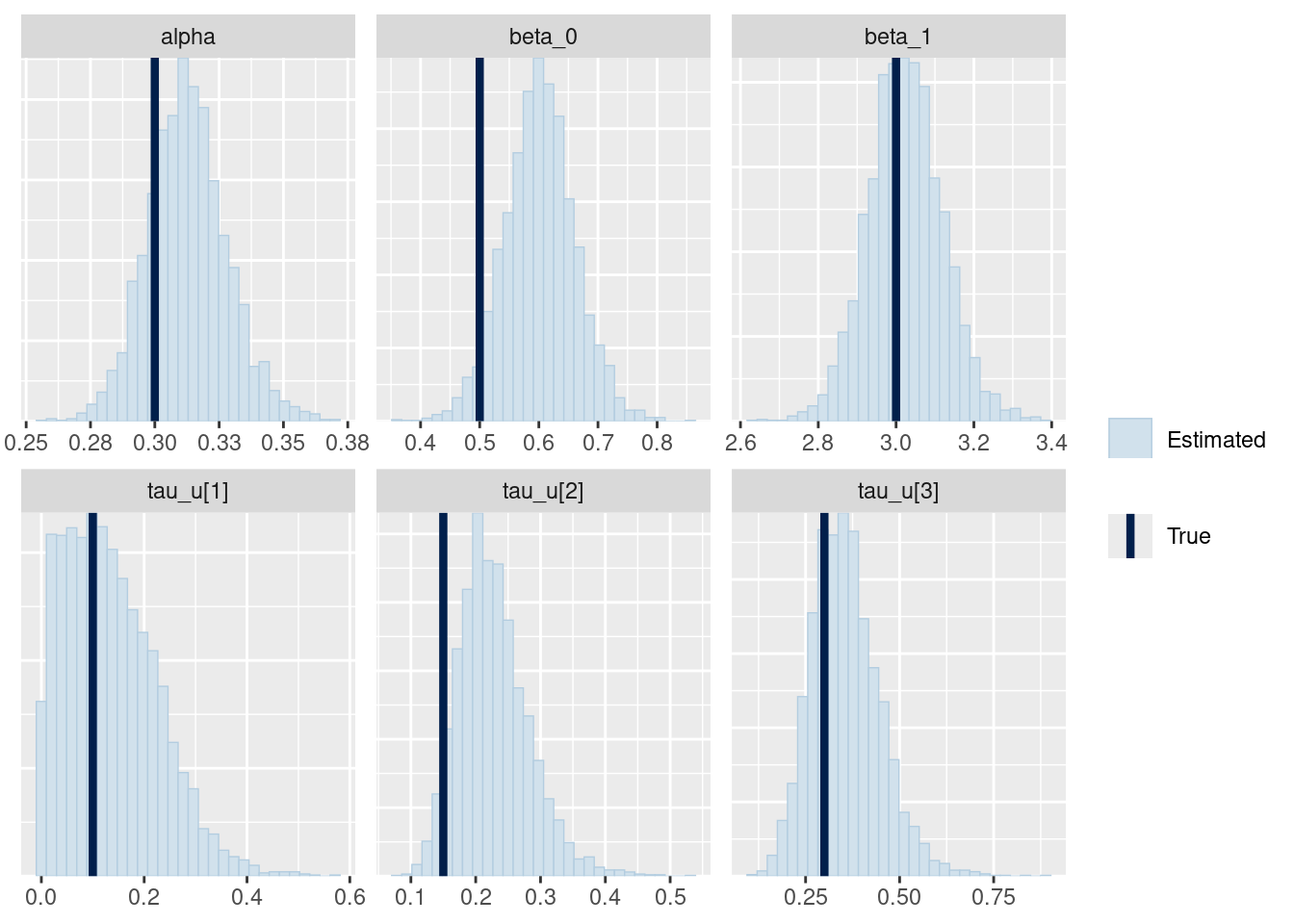
It seems relatively good, but I should probably check it with simulation based calibration (Talts et al. 2018).
Where do we go from here?
One could compare the fit and the predictions of this flavor of Q-learning with another flavor, or with another RL model. The idea would be that each model reflects different theoretical assumptions. It’s also possible to use posterior predictive checks to investigate where the a specific RL model fails and how it should be modified. Finally, RL could be part of a larger model, as in the case of Pedersen, Frank, and Biele (2017), who combined drift diffusion with RL.
Session info 3
sessionInfo()R version 4.3.2 (2023-10-31)
Platform: x86_64-pc-linux-gnu (64-bit)
Running under: Ubuntu 22.04.3 LTS
Matrix products: default
BLAS: /usr/lib/x86_64-linux-gnu/blas/libblas.so.3.10.0
LAPACK: /usr/lib/x86_64-linux-gnu/lapack/liblapack.so.3.10.0
locale:
[1] LC_CTYPE=en_US.UTF-8 LC_NUMERIC=C LC_TIME=nl_NL.UTF-8 LC_COLLATE=en_US.UTF-8 LC_MONETARY=nl_NL.UTF-8
[6] LC_MESSAGES=en_US.UTF-8 LC_PAPER=nl_NL.UTF-8 LC_NAME=C LC_ADDRESS=C LC_TELEPHONE=C
[11] LC_MEASUREMENT=nl_NL.UTF-8 LC_IDENTIFICATION=C
time zone: Europe/Amsterdam
tzcode source: system (glibc)
attached base packages:
[1] stats graphics grDevices utils datasets methods base
other attached packages:
[1] bayesplot_1.10.0 cmdstanr_0.7.1 MASS_7.3-60 extraDistr_1.9.1 ggplot2_3.4.4.9000 purrr_1.0.2 tidyr_1.3.0 dplyr_1.1.3
loaded via a namespace (and not attached):
[1] gtable_0.3.4 tensorA_0.36.2.1 xfun_0.41 bslib_0.5.1 processx_3.8.3 papaja_0.1.2 vctrs_0.6.5
[8] tools_4.3.2 ps_1.7.6 generics_0.1.3 tibble_3.2.1 fansi_1.0.6 highr_0.10 RefManageR_1.4.0
[15] pkgconfig_2.0.3 data.table_1.14.10 checkmate_2.3.1 distributional_0.3.2 assertthat_0.2.1 lifecycle_1.0.4 rcorpora_2.0.0
[22] compiler_4.3.2 farver_2.1.1 stringr_1.5.0 munsell_0.5.0 tinylabels_0.2.4 htmltools_0.5.7 sass_0.4.7
[29] yaml_2.3.7 pillar_1.9.0 crayon_1.5.2 jquerylib_0.1.4 cachem_1.0.8 abind_1.4-5 posterior_1.5.0
[36] tidyselect_1.2.0 digest_0.6.34 stringi_1.8.1 reshape2_1.4.4 bookdown_0.36 labeling_0.4.3 bibtex_0.5.1
[43] fastmap_1.1.1 grid_4.3.2 colorspace_2.1-0 cli_3.6.2 magrittr_2.0.3 emo_0.0.0.9000 utf8_1.2.4
[50] withr_3.0.0 scales_1.3.0 backports_1.4.1 lubridate_1.9.3 timechange_0.2.0 httr_1.4.7 rmarkdown_2.25
[57] matrixStats_1.2.0 blogdown_1.18 evaluate_0.23 knitr_1.45 rlang_1.1.3 Rcpp_1.0.12 glue_1.7.0
[64] xml2_1.3.5 rstudioapi_0.15.0 jsonlite_1.8.8 R6_2.5.1 plyr_1.8.9 References
I actually forgot to bound the parameter at one point, and I could verify that the chains of the MCMC sampler got stuck at different modes.↩︎
I used R (Version 4.3.2; R Core Team 2021) and the R-packages bayesplot (Version 1.10.0; Gabry et al. 2019), cmdstanr (Version 0.7.1; Gabry and Češnovar 2021), dplyr (Version 1.1.3; Wickham et al. 2021), extraDistr (Version 1.9.1; Wolodzko 2020), ggplot2 (Version 3.4.4.9000; Wickham 2016), htmltools (Version 0.5.7; Cheng et al. 2023), knitr (Version 1.45; Xie 2015), purrr (Version 1.0.2; Henry and Wickham 2020), rcorpora (Version 2.0.0; Kazemi et al. 2018), RefManageR (Version 1.4.0; McLean 2017), rmarkdown (Version 2.25; Xie, Allaire, and Grolemund 2018; Xie, Dervieux, and Riederer 2020), and stringr (Version 1.5.0; Wickham 2022) to generate this document.↩︎